Tutorial¶

The following pages show an example analysis with emgfit broken down into the essential steps. Many of the more advanced features of emgfit are left out or only briefly mentioned in passing, so feel free to explore the documentation further!

This tutorial was created in the Jupyter Notebook emgfit_tutorial.ipynb which can be found in the emgfit/emgfit/examples/tutorial/ directory of the emgfit distribution. Feel free to copy the tutorial folder to a different directory (outside of the emgfit/ directory!) and follow along with the tutorial by actually running the code. You can also use this notebook as a template for your own analyses (consider removing some of the explanations). It is recommended to use a separate notebook for each spectrum to be fitted. This enables you to go back to the notebook at any time and check on all the details of how the fits were performed.

emgfit is optimized to be run within Jupyter Notebooks. There is dozens of decent introductions to using Jupyter Notebooks, a nice overview can e.g. be found at https://realpython.com/jupyter-notebook-introduction/. Naturally, the first step of an analysis with emgfit is starting up your notebook server by running jupyter notebook in your command-line interface. This should automatically make the Jupyter interface pop up in a browser window. From there you can navigate to different directories and create a new notebook (new panel on the top right) or open an existing notebook (.ipynb files).

Import the package¶

Assuming you have setup emgfit following the installation instructions, the first step after launching your Jupyter Notebook will be importing the emgfit package:

[1]:

### Import fit package
import emgfit as emg

How to access the documentation¶

Before we actually start processing a spectrum it is important to know how to get access to emgfit’s documentation. There is multiple options for this:

The html documentation can be viewed in any browser. It contains usage examples, detailed explanations of the crucial components and API docs with the different modules and all their methods. The search option and cross references enable quick and easy browsing for help.
Once you have imported emgfit you can access the docs directly from the Jupyter Notebook:
- print all available methods of e.g. the spectrum class by running dir(emg.spectrum)
- print documentation of a method using help(), e.g. the docs of the add_peak method are printed by running help(emg.spectrum.add_peak) in a code cell
- keyboard shortcuts can be even more convenient:
  - Use TAB to get suggestions for auto-completion of method and variable names
  - Place the cursor inside the brackets of a function/method and press SHIFT + TAB to have a window with the function/method documention pop up
  - Pressing the H key inside a Jupyter Notebook shows you all available keyboard shortcuts)

Import data¶

The following code imports the mass data and creates an emgfit spectrum object called spec. The input file must be a TXT or CSV-file following the format of MAc’s hist export mode. From here on the analysis of the spectrum proceeds by calling the various methods on our spectrum object spec.

[2]:

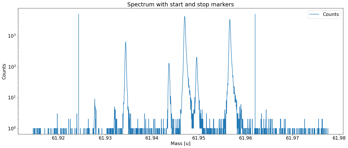
### Import mass data, plot full spectrum and indicate chosen fit range
filename = "2019-09-13_004-_006 SUMMED High stats 62Ga"
skiprows = 38 # number of header rows to skip upon data import
m_start = 61.9243 # low-mass cut off
m_stop = 61.962 # high-mass cut off

spec = emg.spectrum(filename+'.txt',m_start,m_stop,skiprows=skiprows)

Add peaks to the spectrum¶

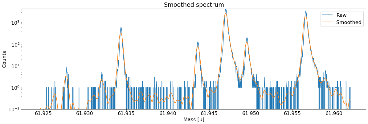
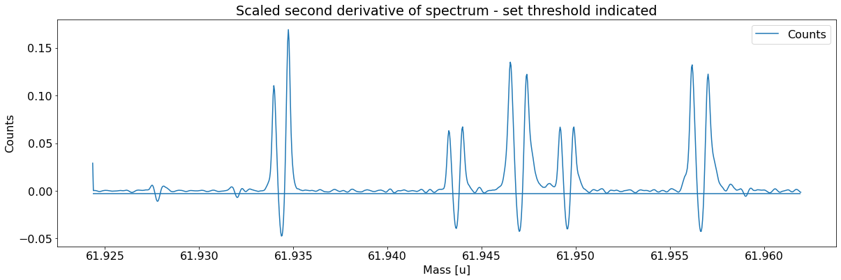
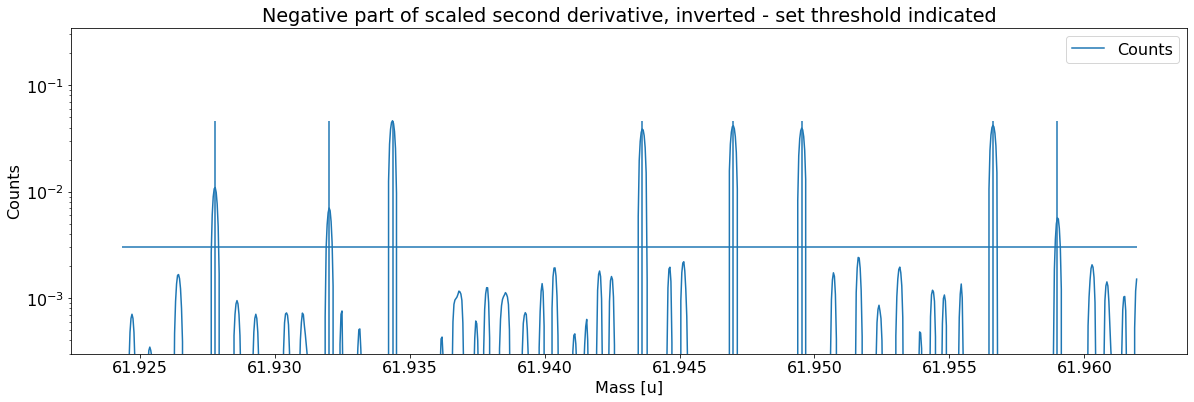
This can be done with the automatic peak detection spectrum method) and/or by manually adding peaks (add_peak spectrum method). The plots shown below are (optional) outputs of the detect_peaks method and depicts the different stages of the automatic peak detection.

All information about the peaks associated with the spectrum are compiled in the peak properties table. The table’s left-most column shows the respective peak indeces. In all fits, the peaks’ x_pos will be used as the initial values for the peak centroid parameters mu (to be exact: mu marks the centroid of the underlying Gaussians).

[3]:

### Detect peaks and add them to spectrum object 'spec'
spec.detect_peaks() # automatic peak detection
#spec.add_peak(61.925,species='?') # manually add a peak at x_pos = 61.925u
#spec.remove_peak(peak_index=0) # manually remove the peak with index 0

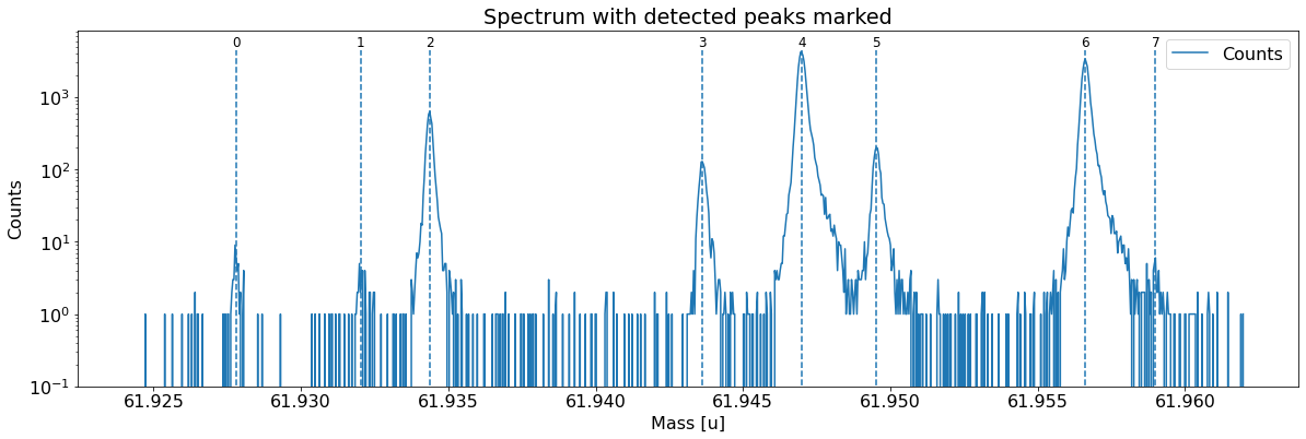
Peak properties table after peak detection:

	x_pos	species	comment	m_AME	m_AME_error	extrapolated	fit_model	cost_func	red_chi	area	area_error	m_ion	rel_stat_error	rel_recal_error	rel_peakshape_error	rel_mass_error	A	atomic_ME_keV	mass_error_keV	m_dev_keV
0	61.927800	?	-	None	None	False	None	None	None	None	None	None	None	None	None	None	None	None	None	None
1	61.932021	?	-	None	None	False	None	None	None	None	None	None	None	None	None	None	None	None	None	None
2	61.934369	?	-	None	None	False	None	None	None	None	None	None	None	None	None	None	None	None	None	None
3	61.943618	?	-	None	None	False	None	None	None	None	None	None	None	None	None	None	None	None	None	None
4	61.946994	?	-	None	None	False	None	None	None	None	None	None	None	None	None	None	None	None	None	None
5	61.949527	?	-	None	None	False	None	None	None	None	None	None	None	None	None	None	None	None	None	None
6	61.956611	?	-	None	None	False	None	None	None	None	None	None	None	None	None	None	None	None	None	None
7	61.958997	?	-	None	None	False	None	None	None	None	None	None	None	None	None	None	None	None	None	None

Assign identified species to the peaks (optional)¶

Although this step is optional, it is highly recommended that it is not skipped. By assigning species labels to your peaks you do not only gain more overview over your spectrum, but also allow for literature values to be automatically fetched from the AME database and entered into the peak properties table. Once a species label has been assigned, you can refer to this peak not only via its index but also via the label.

The assign_species method allows to assign species identifications either to a single selected peak or to all peaks at once. Here the second option was used by passing a list of species labels to assign_species. The list must have the same length as the number of peaks associated with the spectrum object. If there are peaks whose labels should not be changed (e.g. unidentified peaks), simply insert None as a placeholder at the corresponding spots (as done for peaks 2 and 7 below). The syntax for species labels follows MAc’s :-Notation. It is important not to forget to subtract the number of electrons corresponding to the ion’s charge state! Otherwise the analysis would mistakenly proceed with the atomic instead of the ionic mass. Note that currently only singly-charged species are supported by emgfit. Tentative peak identifications can be indicated by adding a '?' to the end of the species string. In this case the literature values are not fetched. The user can also define custom literature values (e.g. to handle isomers or if there are recent measurements that have not entered the AME yet). For more details see the linked documentation of assign_species.

This is also a good point in time to add any comments to the peaks using the add_peak_comment method. These comments can be particularly helpful for the post-processing in Excel since they are written into the output file with the fit results (as is the entire peak properties table). More general comments that concern the entire spectrum can instead be added with the add_spectrum_comment method.

[4]:

### Assign species and add peak comments
spec.assign_species(['Ni62:-1e','Cu62:-1e?',None,'Ga62:-1e','Ti46:O16:-1e','Sc46:O16:-1e','Ca43:F19:-1e',None])
spec.add_peak_comment('Non-isobaric',peak_index=2)
spec.show_peak_properties() # check the changes by printing the peak properties table

Species of peak 0 assigned as Ni62:-1e
Species of peak 1 assigned as Cu62:-1e?
Species of peak 3 assigned as Ga62:-1e
Species of peak 4 assigned as Ti46:O16:-1e
Species of peak 5 assigned as Sc46:O16:-1e
Species of peak 6 assigned as Ca43:F19:-1e
Comment of peak 2 was changed to:  Non-isobaric

	x_pos	species	comment	m_AME	m_AME_error	extrapolated	fit_model	cost_func	red_chi	area	area_error	m_ion	rel_stat_error	rel_recal_error	rel_peakshape_error	rel_mass_error	A	atomic_ME_keV	mass_error_keV	m_dev_keV
0	61.927800	Ni62:-1e	-	61.927796	4.700000e-07	False	None	None	None	None	None	None	None	None	None	None	62.0	None	None	None
1	61.932021	Cu62:-1e?	-	NaN	NaN	False	None	None	None	None	None	None	None	None	None	None	NaN	None	None	None
2	61.934369	?	Non-isobaric	NaN	NaN	False	None	None	None	None	None	None	None	None	None	None	NaN	None	None	None
3	61.943618	Ga62:-1e	-	61.943641	6.940000e-07	False	None	None	None	None	None	None	None	None	None	None	62.0	None	None	None
4	61.946994	Ti46:O16:-1e	-	61.946993	1.760001e-07	False	None	None	None	None	None	None	None	None	None	None	62.0	None	None	None
5	61.949527	Sc46:O16:-1e	-	61.949534	7.320000e-07	False	None	None	None	None	None	None	None	None	None	None	62.0	None	None	None
6	61.956611	Ca43:F19:-1e	-	61.956621	2.440018e-07	False	None	None	None	None	None	None	None	None	None	None	62.0	None	None	None
7	61.958997	?	-	NaN	NaN	False	None	None	None	None	None	None	None	None	None	None	NaN	None	None	None

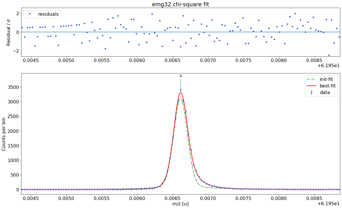
Select the optimal fit model and perform the peak-shape calibration¶

Next we need to find both a fit model and a set of model parameters that capture the shape of our peaks as well as possible. In emgfit both of this is achieved with the determine_peak_shape method. Once the peak-shape calibration has been performed all subsequent fits will be performed with this fixed peak-shape, by only varying the peak centroids, amplitudes and optionally the uniform-baseline parameter bkd_c.

By default determine_peak_shape performs an automatic model selection in which the shape-calibrant peak is first fitted with a pure Gaussian and then with Hyper-EMG functions with an increasing number of expontential tails on the left and right. The algorithm selects the fit model which yields the smallest \(\chi^2_\text{red}\) without having any of the tail weight parameters \(\eta\) compatible with zero within their uncertainty. Alternatively, the auto-model selection can be turned off with the argument vary_tail_order=False and the fit model can be selected manually with the fit_model argument.

Once the best fit model has been selected the method proceeds with the determination of the peak-shape parameters and shows a detailed report with the fit results.

Some recommendations:

It is recommended to do the peak-shape calibration with a chi-squared fit (default) since this yields more robust results and more trusworthy parameter uncertainty estimates. Check the method docs for info on performing the shape calibration with binned maximum likelihood estimation.
Ideally the peak-shape calibration is performed on a well-separated peak with high statistics. In this example, the Ca43:F19:-1e peak was selected as peak-shape calibrant. Since the default fit range includes a smaller peak on the right, the range was manually reduced to 0.45u with the x_fit_range argument. If unavoidable, the peak-shape determination can also be performed on partially overlapping peaks since emgfit ensures identical shape parameters for all peaks being fitted.

[5]:

## Peak-shape calibration with default settings, including automatic model selection:
#spec.determine_peak_shape(species_shape_calib='Ca43:F19:-1e')

## Peak-shape calibration with user-defined fit range:
spec.determine_peak_shape(species_shape_calib='Ca43:F19:-1e',x_fit_range=0.0045)

## Peak-shape calibration with user-defined fit model:
#spec.determine_peak_shape(species_shape_calib='Ca43:F19:-1e',fit_model='emg12',vary_tail_order=False)


##### Determine optimal tail order #####


### Fitting data with Gaussian ###---------------------------------------------------------------------------------------------


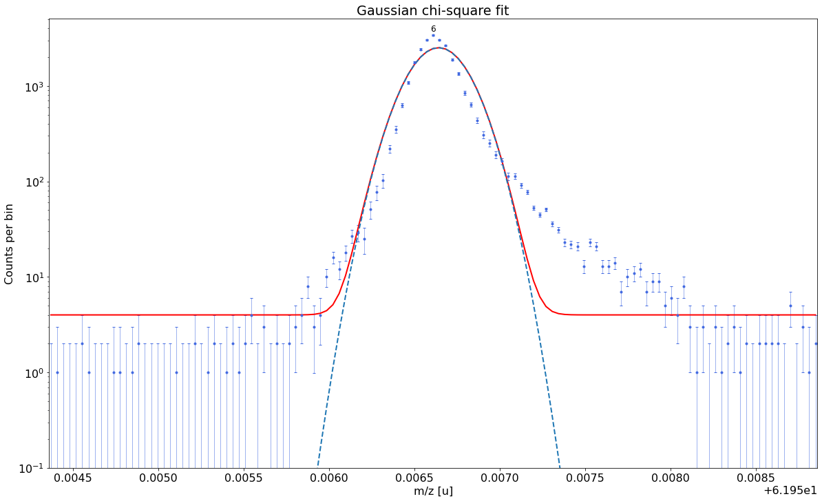
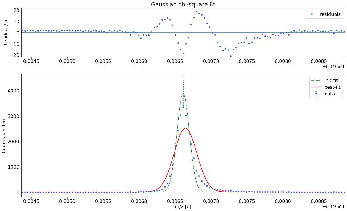
Gaussian-fit yields reduced chi-square of: 45.57 +- 0.13


### Fitting data with emg01 ###---------------------------------------------------------------------------------------------


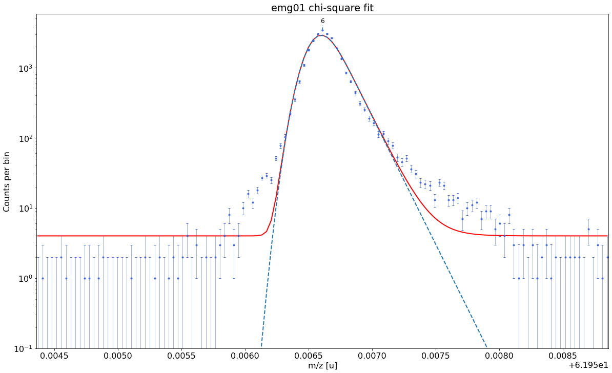
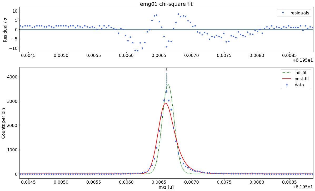
emg01-fit yields reduced chi-square of: 13.79 +- 0.13


### Fitting data with emg10 ###---------------------------------------------------------------------------------------------


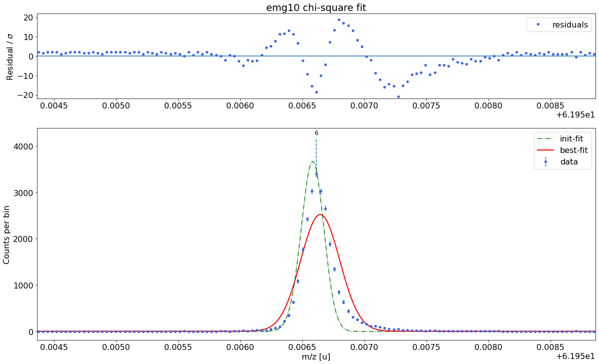
emg10-fit yields reduced chi-square of: 45.96 +- 0.13


### Fitting data with emg11 ###---------------------------------------------------------------------------------------------


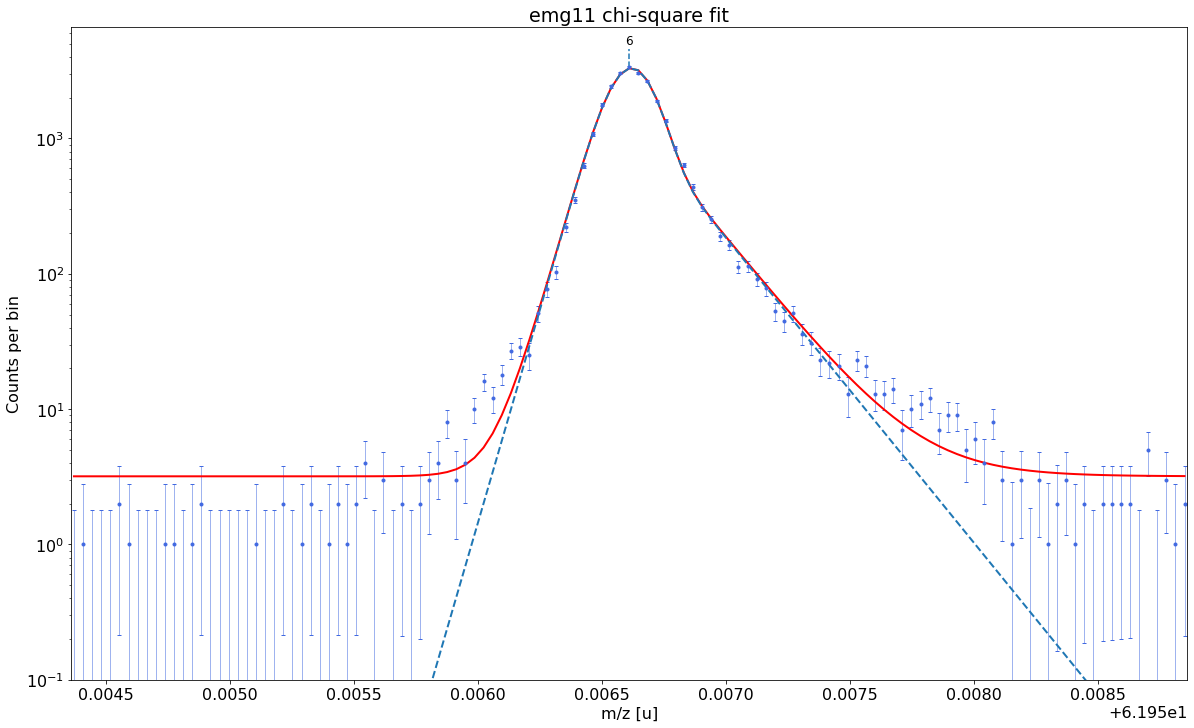
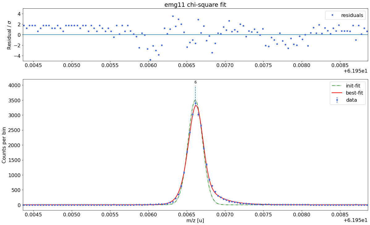
emg11-fit yields reduced chi-square of: 2.6 +- 0.13


### Fitting data with emg12 ###---------------------------------------------------------------------------------------------


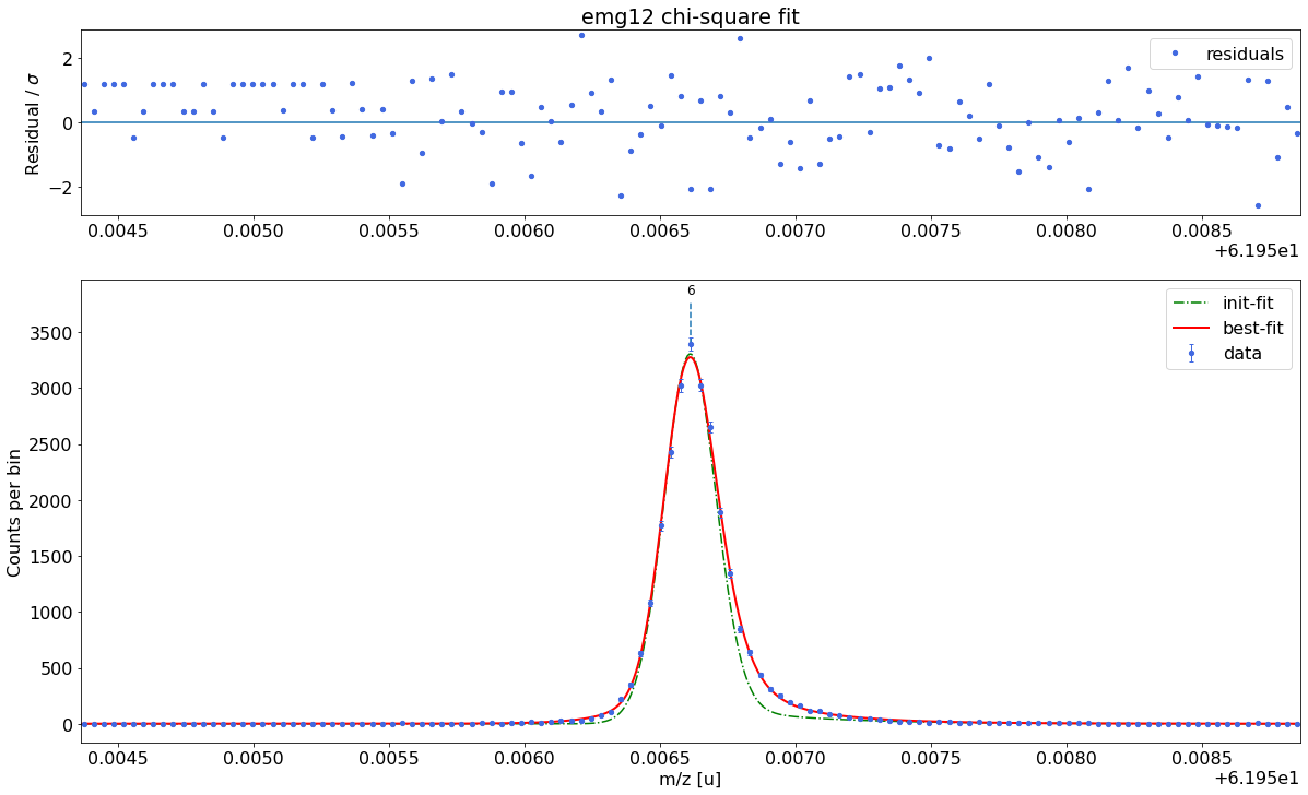
emg12-fit yields reduced chi-square of: 1.22 +- 0.13


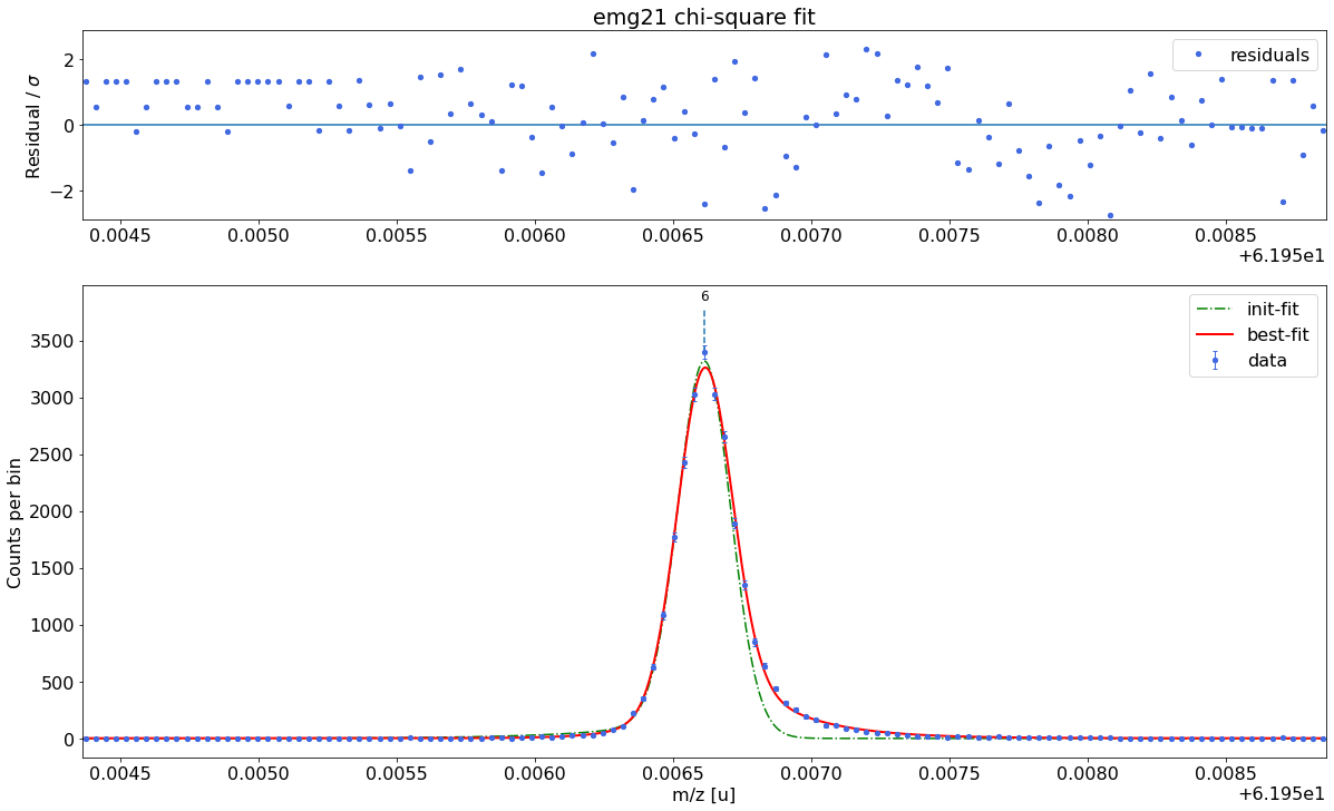
### Fitting data with emg21 ###---------------------------------------------------------------------------------------------

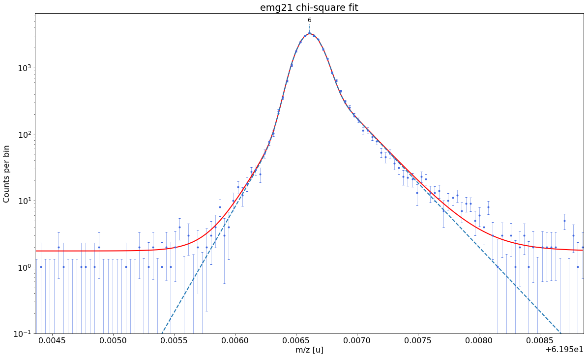
WARNING: p6_eta_m1 = 0.901 +- 0.987  is compatible with zero within uncertainty.
             This tail order is likely overfitting the data and will be excluded from selection.
WARNING: p6_eta_m2 = 0.099 +- 0.987  is compatible with zero within uncertainty.
             This tail order is likely overfitting the data and will be excluded from selection.

emg21-fit yields reduced chi-square of: 1.47 +- 0.13


### Fitting data with emg22 ###---------------------------------------------------------------------------------------------


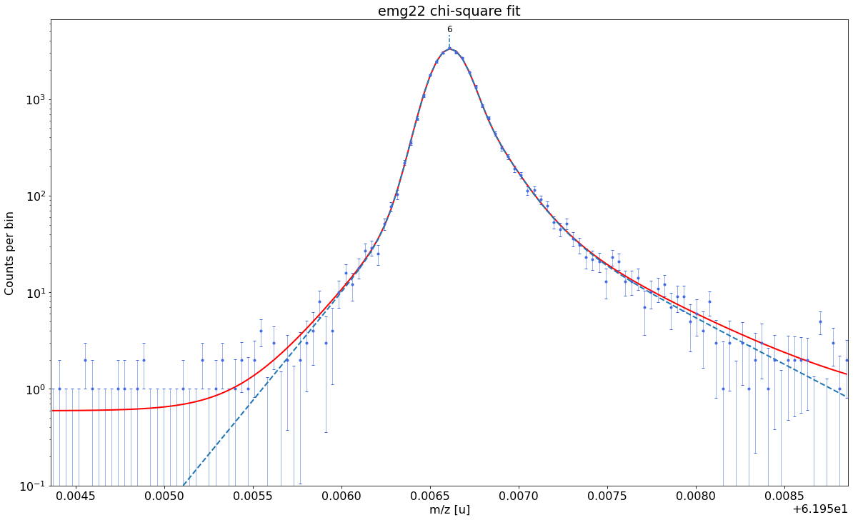
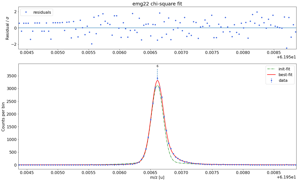
emg22-fit yields reduced chi-square of: 0.93 +- 0.13


### Fitting data with emg23 ###---------------------------------------------------------------------------------------------

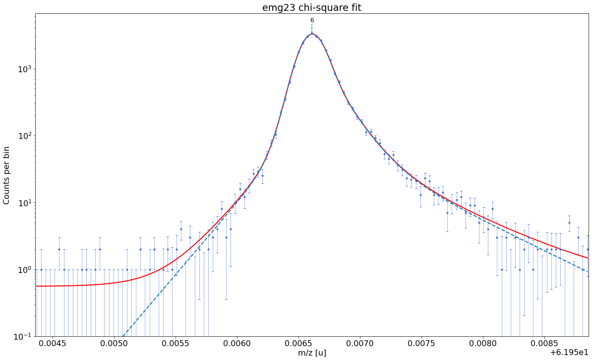
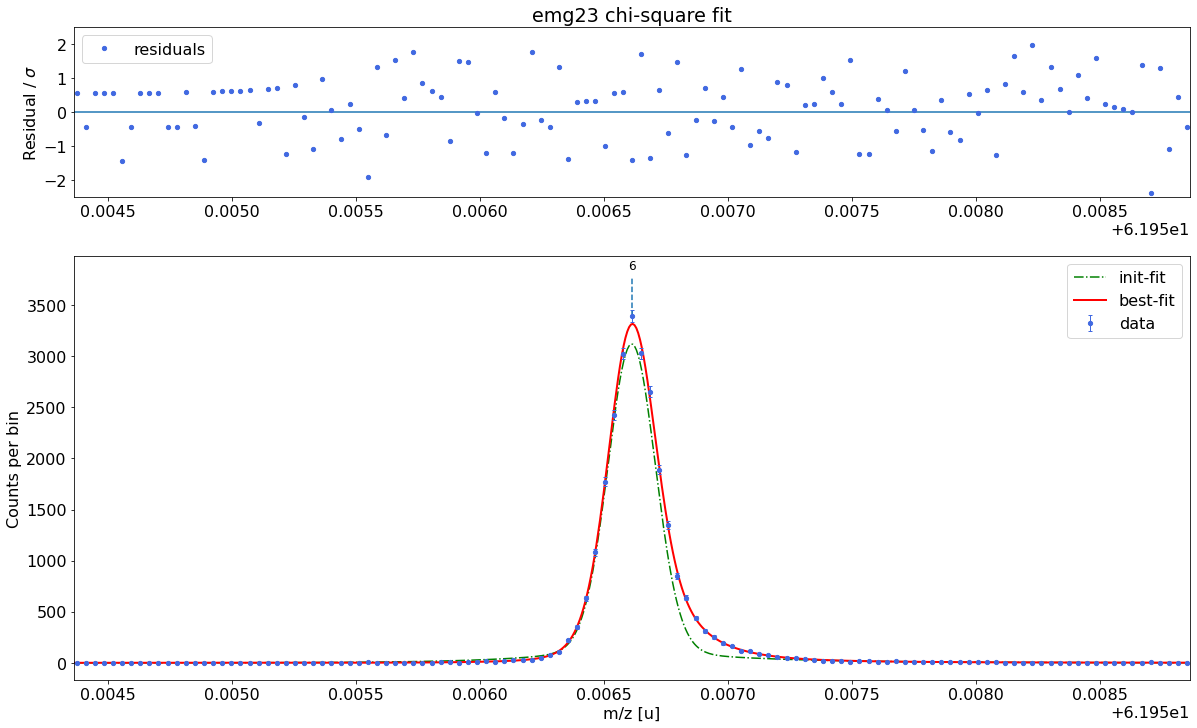
WARNING: p6_eta_m1 = 0.902 +- 0.916  is compatible with zero within uncertainty.
             This tail order is likely overfitting the data and will be excluded from selection.
WARNING: p6_eta_m2 = 0.098 +- 0.916  is compatible with zero within uncertainty.
             This tail order is likely overfitting the data and will be excluded from selection.
WARNING: p6_eta_p1 = 0.482 +- 2.46  is compatible with zero within uncertainty.
             This tail order is likely overfitting the data and will be excluded from selection.
WARNING: p6_eta_p2 = 0.438 +- 1.894  is compatible with zero within uncertainty.
             This tail order is likely overfitting the data and will be excluded from selection.
WARNING: p6_eta_p3 = 0.08 +- 2.46  is compatible with zero within uncertainty.
             This tail order is likely overfitting the data and will be excluded from selection.

emg23-fit yields reduced chi-square of: 0.94 +- 0.13


### Fitting data with emg32 ###---------------------------------------------------------------------------------------------

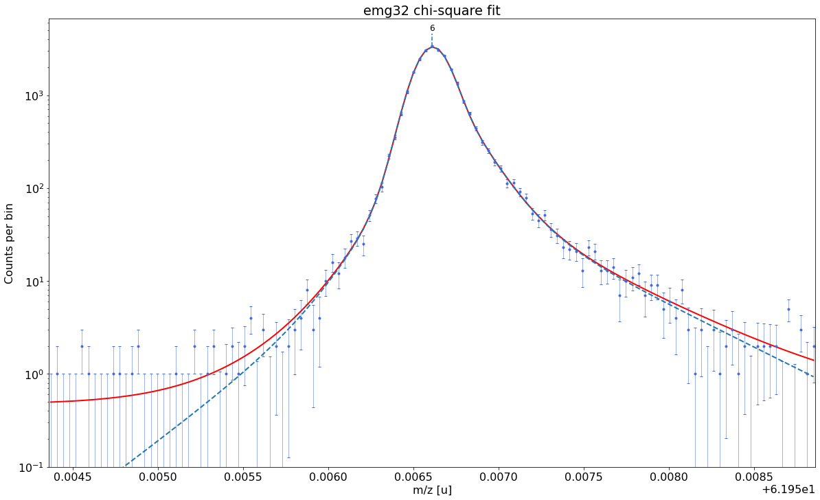
WARNING: p6_eta_m2 = 0.015 +- 0.076  is compatible with zero within uncertainty.
             This tail order is likely overfitting the data and will be excluded from selection.
WARNING: p6_eta_m3 = 0.095 +- 0.133  is compatible with zero within uncertainty.
             This tail order is likely overfitting the data and will be excluded from selection.

emg32-fit yields reduced chi-square of: 0.94 +- 0.13


### Fitting data with emg33 ###---------------------------------------------------------------------------------------------

WARNING: p6_eta_m1 = 0.863 +- 4.743  is compatible with zero within uncertainty.
             This tail order is likely overfitting the data and will be excluded from selection.
WARNING: p6_eta_m2 = 0.116 +- 3.916  is compatible with zero within uncertainty.
             This tail order is likely overfitting the data and will be excluded from selection.
WARNING: p6_eta_m3 = 0.02 +- 4.743  is compatible with zero within uncertainty.
             This tail order is likely overfitting the data and will be excluded from selection.
WARNING: p6_eta_p1 = 0.475 +- 11.47  is compatible with zero within uncertainty.
             This tail order is likely overfitting the data and will be excluded from selection.
WARNING: p6_eta_p2 = 0.447 +- 8.983  is compatible with zero within uncertainty.
             This tail order is likely overfitting the data and will be excluded from selection.
WARNING: p6_eta_p3 = 0.078 +- 11.47  is compatible with zero within uncertainty.
             This tail order is likely overfitting the data and will be excluded from selection.

emg33-fit yields reduced chi-square of: 0.96 +- 0.14


##### RESULT OF AUTOMATIC MODEL SELECTION: #####

    Best fit model determined to be: emg22
    Corresponding chi²-reduced: 0.93


##### Peak-shape determination #####-------------------------------------------------------------------------------------------

Model

(Model(constant, prefix='bkg_') + Model(emg22, prefix='p6_'))

Fit Statistics

fitting method	least_squares
# function evals	16
# data points	123
# variables	11
chi-square	104.451674
reduced chi-square	0.93260424
Akaike info crit.	1.89444012
Bayesian info crit.	32.8284680

Variables

name	value	standard error	relative error	initial value	min	max	vary	expression
bkg_c	0.59386072	0.19767135	(33.29%)	0.1	0.00000000	4.00000000	True
p6_amp	0.95323437	0.00599104	(0.63%)	0.8422080000000001	1.0000e-20	inf	True
p6_mu	61.9566409	3.6332e-06	(0.00%)	61.95661076349748	61.9466108	61.9666108	True
p6_sigma	8.3298e-05	2.7262e-06	(3.27%)	8.68e-05	0.00000000	0.00508680	True
p6_theta	0.72958107	0.02084641	(2.86%)	0.5	0.00000000	1.00000000	True
p6_eta_m1	0.93085594	0.01775570	(1.91%)	0.85	0.00000000	1.00000000	True
p6_eta_m2	0.06914406	0.01775570	(25.68%)	0.15000000000000002	0.00000000	1.00000000	False	1-p6_eta_m1
p6_tau_m1	4.6426e-05	5.0748e-06	(10.93%)	3.1e-05	1.0000e-12	0.05000000	True
p6_tau_m2	1.9392e-04	2.5525e-05	(13.16%)	0.00031	1.0000e-12	0.05000000	True
p6_eta_p1	0.81292600	0.03620254	(4.45%)	0.85	0.00000000	1.00000000	True
p6_eta_p2	0.18707400	0.03620254	(19.35%)	0.15000000000000002	0.00000000	1.00000000	False	1-p6_eta_p1
p6_tau_p1	1.2908e-04	1.1799e-05	(9.14%)	3.1e-05	1.0000e-12	0.05000000	True
p6_tau_p2	4.5400e-04	5.9304e-05	(13.06%)	0.000372	1.0000e-12	0.05000000	True

Correlations (unreported correlations are < 0.100)

p6_eta_m1	p6_tau_m2	0.9372
p6_eta_p1	p6_tau_p2	0.9072
p6_theta	p6_tau_p1	0.8344
p6_sigma	p6_tau_m1	-0.8097
p6_eta_m1	p6_tau_m1	0.7516
p6_tau_p1	p6_tau_p2	0.7466
p6_eta_p1	p6_tau_p1	0.7019
p6_mu	p6_tau_m1	0.6956
p6_tau_m1	p6_tau_m2	0.6790
p6_sigma	p6_theta	0.6079
p6_mu	p6_eta_m1	0.5919
p6_mu	p6_theta	0.5288
p6_sigma	p6_tau_p1	0.5241
bkg_c	p6_tau_m2	-0.5166
p6_mu	p6_tau_m2	0.4970
p6_theta	p6_tau_p2	0.4598
bkg_c	p6_eta_m1	-0.4054
p6_sigma	p6_eta_m1	-0.3891
bkg_c	p6_tau_p2	-0.3828
p6_sigma	p6_tau_m2	-0.3734
p6_mu	p6_tau_p1	0.3515
p6_theta	p6_eta_p1	0.3051
p6_mu	p6_tau_p2	0.2685
p6_mu	p6_sigma	-0.2643
bkg_c	p6_tau_m1	-0.2445
p6_tau_m1	p6_tau_p1	-0.2418
bkg_c	p6_eta_p1	-0.2295
bkg_c	p6_mu	-0.2220
p6_sigma	p6_tau_p2	0.2164
p6_theta	p6_tau_m1	-0.1912
p6_mu	p6_eta_p1	0.1583
p6_tau_m2	p6_tau_p2	0.1564
bkg_c	p6_amp	-0.1405
bkg_c	p6_tau_p1	-0.1399
p6_eta_m1	p6_tau_p2	0.1367
p6_sigma	p6_eta_p1	0.1142

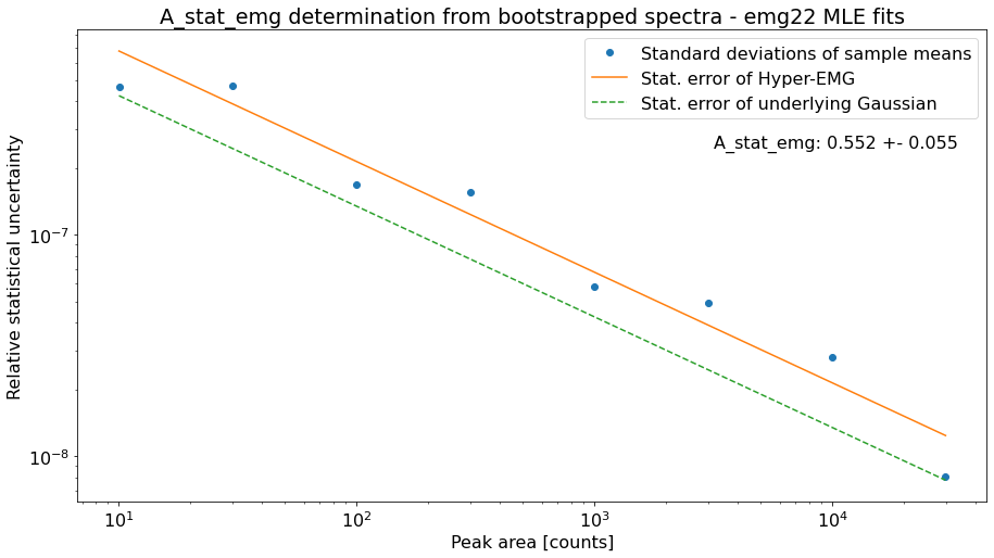
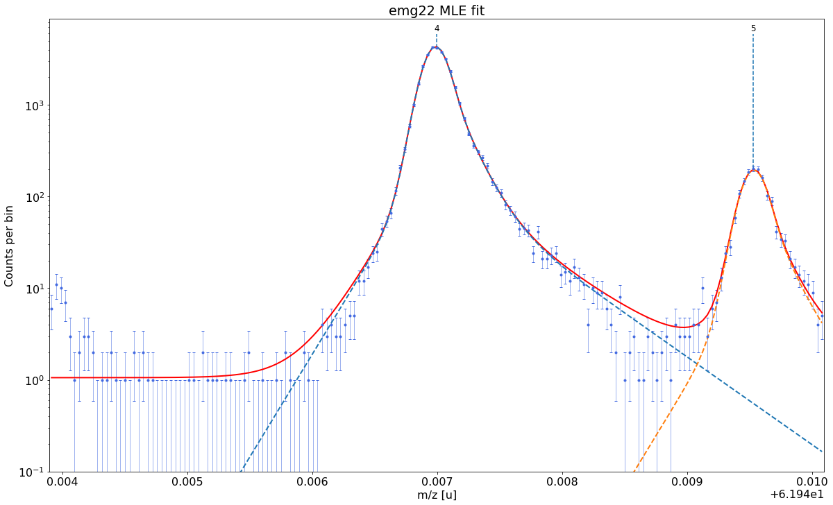
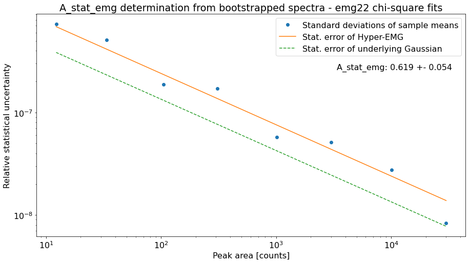
Determine A_stat_emg for subsequent stat. error estimations (optional)¶

The statistical uncertainties of Hyper-EMG fits are estimated using the equation:

\(\sigma_{stat} = A_{stat,emg} \cdot \frac{\mathrm{FWHM}}{\sqrt{N_{counts}}}\)

where \(\mathrm{FWHM}\) and \(N_{counts}\) refer to the full width at half maximum and the number of counts in the respective peak.

By default a of value \(A_{stat,emg} = 0.52\) will be used for Hyper-EMG models (for Gaussians \(A_{stat,G}=0.425\)).

However, \(A_{stat,emg}\) depends on the peak-shape and can deviate from the default value. Therefore, the determine_A_stat_emg method can be used to estimate \(A_{stat,emg}\) for the specific peak shape in the spectrum. This is done by fitting many simulated spectra created via bootstrap re-sampling from a reference peak in the spectrum. The reference peak should be well-separated and have decent statistics (e.g. the peak-shape calibrant). For details on how \(A_{stat,emg}\) is estimated see the linked docs of determine_A_stat_emg.

This method will typically run for ~10 minutes if N_spectra=1000 (default) is used. Since this is only for demonstration purposes the number of bootstrapped spectra generated for each data point (N_spectra argument) was reduced to 10 to get a quicker run time. This is also the reason for the large scatter of the data points below.

In practice it is convenient to skip this method for the first processing of the spectrum since this will only affect the statistical uncertainties but no other fit properties. Once reasonable fits have been achieved for all peaks of interest in the cells below, the exact uncertainties can be obtained by returning to this cell to execute determine_A_stat_emg with a decent value for N_spectra and then re-runnning the cells below (then with the update value for determine_A_stat_emg). The latter is conveniently done by using the Run All Below option in the Cell panel of the Jupyter Notebook.

[6]:

# Determine A_stat_emg and save the resulting plot
spec.determine_A_stat_emg(species='Ca43:F19:-1e',x_range=0.004,plot_filename='outputs/'+filename+'_MLE',N_spectra=10)

Creating synthetic spectra via bootstrap re-sampling and fitting  them for A_stat determination.
Depending on the choice of `N_spectra` this can take a few minutes. Interrupt kernel if this takes too long.


Done!

[[Model]]
    Model(powerlaw)
[[Fit Statistics]]
    # fitting method   = leastsq
    # function evals   = 5
    # data points      = 8
    # variables        = 1
    chi-square         = 9.6122e-09
    reduced chi-square = 1.3732e-09
    Akaike info crit   = -162.317379
    Bayesian info crit = -162.237937
[[Variables]]
    amplitude:  1.3260e-04 +/- 1.3094e-05 (9.87%) (init = 1)
    exponent:  -0.5 (fixed)

A_stat of a Gaussian model: 0.425
Default A_stat_emg for Hyper-EMG models: 0.52
A_stat_emg for this spectrum's emg22 fit model: 0.552 +- 0.055

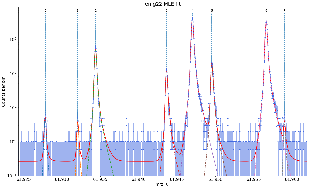
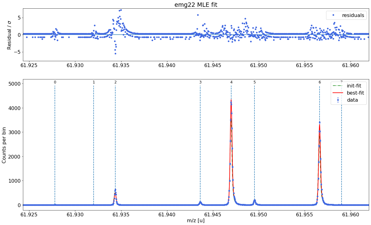
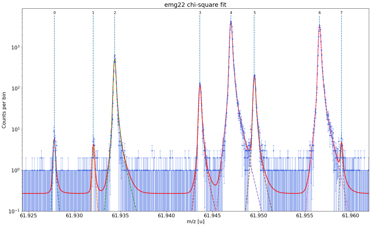
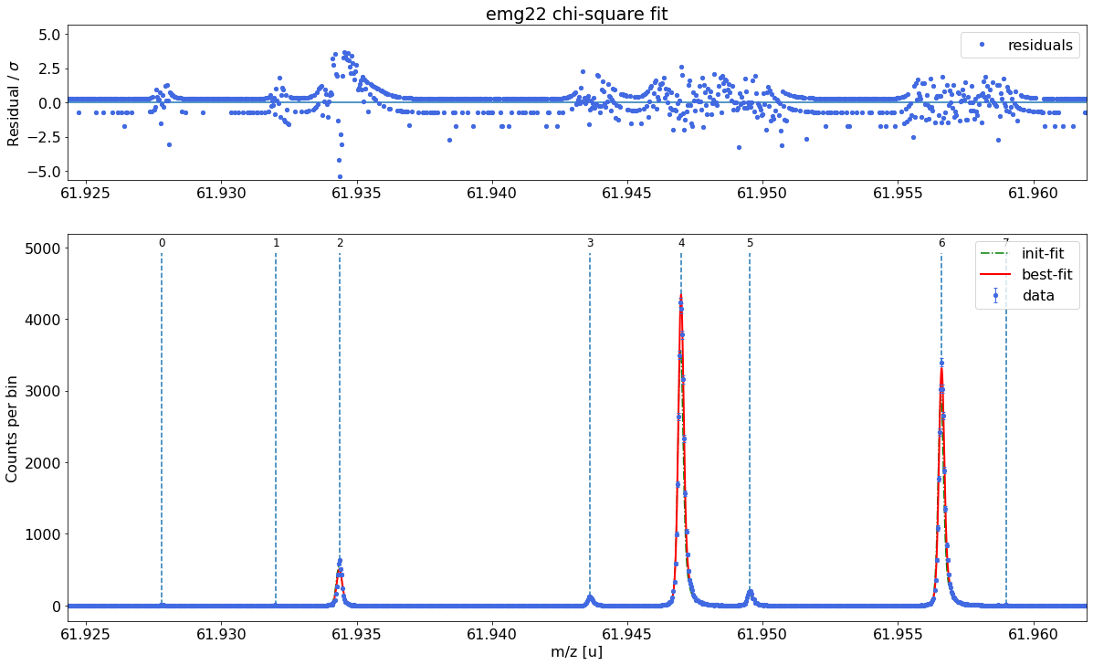
Fit all peaks, perform mass re-calibration & obtain final mass values¶

The following code fits all peaks in the spectrum, performs the mass (re-)calibration, determines the peak-shape uncertainties and updates the peak properties list with the results including the final mass values and their uncertainties.

The simultaneous mass recalibration is optional and only invoked when the species_mass_calib (or the index_mass_calib) argument are specified. If this feature is not used, the fit_peaks method requires a pre-existing mass calibration (see Alternative 1 section below). In contrast to determine_peak_shape, by default fit_peaks performs a binned maximum likelihood fit (‘MLE’). For chi-square fitting with fit_peaks see Alternative 2 section below. Fits with fit_peaks can be restricted to a user-defined mass range (see the commented-out line of code below).

[7]:

# Maximum likelihood fit of all peaks in the spectrum
spec.fit_peaks(species_mass_calib='Ti46:O16:-1e')

# Maximum likelihood fit of peaks in a user-defined mass range
#spec.fit_peaks(species_mass_calib='Ti46:O16:-1e',x_fit_cen=61.9455,x_fit_range=0.01)


##### Mass recalibration #####


Relative literature error of mass calibrant:    3e-09
Relative statistical error of mass calibrant:   1.2e-08

Recalibration factor:      0.999999689 = 1 -3.11e-07
Relative recalibration error:  1.2e-08


##### Peak-shape uncertainty evaluation #####

All mass shifts below are corrected for the corresponding shifts of the calibrant peak.

Determining absolute centroid shifts of mass calibrant.

Re-fitting with sigma = 8.33e-05 +/- 2.73e-06 shifts peak 0 by -0.215 /  0.168 μu.
Re-fitting with sigma = 8.33e-05 +/- 2.73e-06 shifts peak 1 by  0.454 / -0.406 μu.
Re-fitting with sigma = 8.33e-05 +/- 2.73e-06 shifts peak 2 by -0.387 /  0.217 μu.
Re-fitting with sigma = 8.33e-05 +/- 2.73e-06 shifts peak 3 by -0.037 /  0.010 μu.
Re-fitting with sigma = 8.33e-05 +/- 2.73e-06 shifts peak 5 by  0.016 / -0.084 μu.
Re-fitting with sigma = 8.33e-05 +/- 2.73e-06 shifts peak 6 by  0.036 / -0.018 μu.
Re-fitting with sigma = 8.33e-05 +/- 2.73e-06 shifts peak 7 by  0.212 / -0.204 μu.

Re-fitting with theta = 7.30e-01 +/- 2.08e-02 shifts peak 0 by -0.459 /  0.392 μu.
Re-fitting with theta = 7.30e-01 +/- 2.08e-02 shifts peak 1 by -0.912 /  0.933 μu.
Re-fitting with theta = 7.30e-01 +/- 2.08e-02 shifts peak 2 by -0.443 /  0.224 μu.
Re-fitting with theta = 7.30e-01 +/- 2.08e-02 shifts peak 3 by -0.164 /  0.142 μu.
Re-fitting with theta = 7.30e-01 +/- 2.08e-02 shifts peak 5 by -0.167 /  0.250 μu.
Re-fitting with theta = 7.30e-01 +/- 2.08e-02 shifts peak 6 by -0.096 /  0.068 μu.
Re-fitting with theta = 7.30e-01 +/- 2.08e-02 shifts peak 7 by -1.599 /  1.712 μu.

Re-fitting with eta_m1 = 9.31e-01 +/- 1.78e-02 shifts peak 0 by  0.519 / -0.521 μu.
Re-fitting with eta_m1 = 9.31e-01 +/- 1.78e-02 shifts peak 1 by  0.306 / -0.241 μu.
Re-fitting with eta_m1 = 9.31e-01 +/- 1.78e-02 shifts peak 2 by  0.212 / -0.433 μu.
Re-fitting with eta_m1 = 9.31e-01 +/- 1.78e-02 shifts peak 3 by  0.271 / -0.209 μu.
Re-fitting with eta_m1 = 9.31e-01 +/- 1.78e-02 shifts peak 5 by  0.229 / -0.170 μu.
Re-fitting with eta_m1 = 9.31e-01 +/- 1.78e-02 shifts peak 6 by  0.070 / -0.064 μu.
Re-fitting with eta_m1 = 9.31e-01 +/- 1.78e-02 shifts peak 7 by  0.445 / -0.345 μu.

Re-fitting with tau_m1 = 4.64e-05 +/- 5.07e-06 shifts peak 0 by -0.697 /  0.700 μu.
Re-fitting with tau_m1 = 4.64e-05 +/- 5.07e-06 shifts peak 1 by  0.211 / -0.210 μu.
Re-fitting with tau_m1 = 4.64e-05 +/- 5.07e-06 shifts peak 2 by -0.516 /  0.354 μu.
Re-fitting with tau_m1 = 4.64e-05 +/- 5.07e-06 shifts peak 3 by -0.085 /  0.136 μu.
Re-fitting with tau_m1 = 4.64e-05 +/- 5.07e-06 shifts peak 5 by -0.140 /  0.082 μu.
Re-fitting with tau_m1 = 4.64e-05 +/- 5.07e-06 shifts peak 6 by -0.046 / -0.036 μu.
Re-fitting with tau_m1 = 4.64e-05 +/- 5.07e-06 shifts peak 7 by -0.739 /  0.706 μu.

Re-fitting with tau_m2 = 1.94e-04 +/- 2.55e-05 shifts peak 0 by -0.257 /  0.245 μu.
Re-fitting with tau_m2 = 1.94e-04 +/- 2.55e-05 shifts peak 1 by -0.149 /  0.124 μu.
Re-fitting with tau_m2 = 1.94e-04 +/- 2.55e-05 shifts peak 2 by -0.269 /  0.027 μu.
Re-fitting with tau_m2 = 1.94e-04 +/- 2.55e-05 shifts peak 3 by -0.132 /  0.191 μu.
Re-fitting with tau_m2 = 1.94e-04 +/- 2.55e-05 shifts peak 5 by -0.063 /  0.156 μu.
Re-fitting with tau_m2 = 1.94e-04 +/- 2.55e-05 shifts peak 6 by -0.044 /  0.052 μu.
Re-fitting with tau_m2 = 1.94e-04 +/- 2.55e-05 shifts peak 7 by  0.200 / -0.031 μu.

Re-fitting with eta_p1 = 8.13e-01 +/- 3.62e-02 shifts peak 0 by -0.044 / -0.033 μu.
Re-fitting with eta_p1 = 8.13e-01 +/- 3.62e-02 shifts peak 1 by -0.210 /  0.088 μu.
Re-fitting with eta_p1 = 8.13e-01 +/- 3.62e-02 shifts peak 2 by -0.166 / -0.038 μu.
Re-fitting with eta_p1 = 8.13e-01 +/- 3.62e-02 shifts peak 3 by -0.102 /  0.073 μu.
Re-fitting with eta_p1 = 8.13e-01 +/- 3.62e-02 shifts peak 5 by -0.223 /  0.179 μu.
Re-fitting with eta_p1 = 8.13e-01 +/- 3.62e-02 shifts peak 6 by  0.027 / -0.012 μu.
Re-fitting with eta_p1 = 8.13e-01 +/- 3.62e-02 shifts peak 7 by -3.045 /  2.414 μu.

Re-fitting with tau_p1 = 1.29e-04 +/- 1.18e-05 shifts peak 0 by  0.005 / -0.140 μu.
Re-fitting with tau_p1 = 1.29e-04 +/- 1.18e-05 shifts peak 1 by  0.230 / -0.364 μu.
Re-fitting with tau_p1 = 1.29e-04 +/- 1.18e-05 shifts peak 2 by  0.175 / -0.513 μu.
Re-fitting with tau_p1 = 1.29e-04 +/- 1.18e-05 shifts peak 3 by  0.129 / -0.193 μu.
Re-fitting with tau_p1 = 1.29e-04 +/- 1.18e-05 shifts peak 5 by  0.026 / -0.008 μu.
Re-fitting with tau_p1 = 1.29e-04 +/- 1.18e-05 shifts peak 6 by -0.023 / -0.001 μu.
Re-fitting with tau_p1 = 1.29e-04 +/- 1.18e-05 shifts peak 7 by  0.428 / -0.476 μu.

Re-fitting with tau_p2 = 4.54e-04 +/- 5.93e-05 shifts peak 0 by -0.082 /  0.058 μu.
Re-fitting with tau_p2 = 4.54e-04 +/- 5.93e-05 shifts peak 1 by  0.315 / -0.341 μu.
Re-fitting with tau_p2 = 4.54e-04 +/- 5.93e-05 shifts peak 2 by  0.009 / -0.035 μu.
Re-fitting with tau_p2 = 4.54e-04 +/- 5.93e-05 shifts peak 3 by  0.024 / -0.042 μu.
Re-fitting with tau_p2 = 4.54e-04 +/- 5.93e-05 shifts peak 5 by  0.367 / -0.460 μu.
Re-fitting with tau_p2 = 4.54e-04 +/- 5.93e-05 shifts peak 6 by -0.041 /  0.030 μu.
Re-fitting with tau_p2 = 4.54e-04 +/- 5.93e-05 shifts peak 7 by  1.360 / -6.339 μu.

Relative peak-shape error of peak 0: 1.7e-08
Relative peak-shape error of peak 1: 2e-08
Relative peak-shape error of peak 2: 1.7e-08
Relative peak-shape error of peak 3: 7e-09
Relative peak-shape error of peak 5: 1.1e-08
Relative peak-shape error of peak 6: 2e-09
Relative peak-shape error of peak 7: 1.18e-07

	x_pos	species	comment	m_AME	m_AME_error	extrapolated	fit_model	cost_func	red_chi	area	area_error	m_ion	rel_stat_error	rel_recal_error	rel_peakshape_error	rel_mass_error	A	atomic_ME_keV	mass_error_keV	m_dev_keV
0	61.927800	Ni62:-1e	-	61.927796	4.700000e-07	False	emg22	MLE	1.22	38.67	6.77	61.927795	3.443261e-07	1.195055e-08	1.703021e-08	3.449541e-07	62.0	-66747.110	19.898804	-0.780
1	61.932021	Cu62:-1e?	-	NaN	NaN	False	emg22	MLE	1.22	28.07	5.98	61.932051	4.041159e-07	1.195055e-08	1.996842e-08	4.047854e-07	NaN	NaN	23.351804	NaN
2	61.934369	?	Non-isobaric	NaN	NaN	False	emg22	MLE	1.22	3872.82	62.56	61.934369	3.440307e-08	1.195055e-08	1.742012e-08	4.037137e-08	NaN	NaN	2.329085	NaN
3	61.943618	Ga62:-1e	-	61.943641	6.940000e-07	False	emg22	MLE	1.22	954.58	31.20	61.943636	6.928509e-08	1.195055e-08	7.319824e-09	7.068818e-08	62.0	-51992.051	4.078717	-5.139
4	61.946994	Ti46:O16:-1e	mass calibrant	61.946993	1.760001e-07	False	emg22	MLE	1.22	34004.53	186.60	61.946993	1.160791e-08	1.195055e-08	NaN	NaN	62.0	-48864.806	NaN	0.000
5	61.949527	Sc46:O16:-1e	-	61.949534	7.320000e-07	False	emg22	MLE	1.22	1567.77	40.11	61.949540	5.405842e-08	1.195055e-08	1.055765e-08	5.636127e-08	62.0	-46492.209	3.252363	6.017
6	61.956611	Ca43:F19:-1e	shape calibrant	61.956621	2.440018e-07	False	emg22	MLE	1.22	25966.02	161.32	61.956622	1.328166e-08	1.195055e-08	2.466068e-09	1.803606e-08	62.0	-39895.679	1.040901	0.593
7	61.958997	?	-	NaN	NaN	False	emg22	MLE	1.22	25.28	6.40	61.959019	4.256470e-07	1.195055e-08	1.179912e-07	4.418598e-07	NaN	NaN	25.501701	NaN

The values for chi-squared as well as the parameter uncertainties and correlations reported by lmfit below should be taken with caution when your MLE fit includes bins with low statistics. For details see Notes section in the spectrum.peakfit() method documentation.

Model

((((((((Model(constant, prefix='bkg_') + Model(emg22, prefix='p0_')) + Model(emg22, prefix='p1_')) + Model(emg22, prefix='p2_')) + Model(emg22, prefix='p3_')) + Model(emg22, prefix='p4_')) + Model(emg22, prefix='p5_')) + Model(emg22, prefix='p6_')) + Model(emg22, prefix='p7_'))

Fit Statistics

fitting method	least_squares
# function evals	9
# data points	1027
# variables	17
chi-square	1237.06416
reduced chi-square	1.22481600
Akaike info crit.	225.123700
Bayesian info crit.	309.008452

Variables

name	value	standard error	relative error	initial value	min	max	vary	expression
bkg_c	0.26119680	0.02315482	(8.86%)	0.1	0.00000000	4.00000000	True
p0_amp	0.00141907	2.4842e-04	(17.51%)	0.001488	1.0000e-20	inf	True
p0_mu	61.9278147	2.2955e-05	(0.00%)	61.927800309876424	61.9178003	61.9378003	True
p0_sigma	8.3298e-05	0.00000000	(0.00%)	8.329830944305415e-05	0.00000000	0.00508330	False
p0_theta	0.72958107	0.00000000	(0.00%)	0.7295810682165222	0.00000000	1.00000000	False
p0_eta_m1	0.93085594	0.00000000	(0.00%)	0.9308559436145877	0.00000000	1.00000000	False
p0_eta_m2	0.06914406	0.00000000	(0.00%)	0.06914405638541232	0.00000000	1.00000000	False	1-p0_eta_m1
p0_tau_m1	4.6426e-05	0.00000000	(0.00%)	4.6426492114914925e-05	1.0000e-12	0.05000000	False
p0_tau_m2	1.9392e-04	0.00000000	(0.00%)	0.0001939165239395595	1.0000e-12	0.05000000	False
p0_eta_p1	0.81292600	0.00000000	(0.00%)	0.8129260035354914	0.00000000	1.00000000	False
p0_eta_p2	0.18707400	0.00000000	(0.00%)	0.18707399646450862	0.00000000	1.00000000	False	1-p0_eta_p1
p0_tau_p1	1.2908e-04	0.00000000	(0.00%)	0.0001290811175724487	1.0000e-12	0.05000000	False
p0_tau_p2	4.5400e-04	0.00000000	(0.00%)	0.0004539974092137846	1.0000e-12	0.05000000	False
p1_amp	0.00103012	2.1954e-04	(21.31%)	0.000496	1.0000e-20	inf	True
p1_mu	61.9320700	2.7212e-05	(0.00%)	61.93202053070152	61.9220205	61.9420205	True
p1_sigma	8.3298e-05	0.00000000	(0.00%)	8.329830944305415e-05	0.00000000	0.00508330	False
p1_theta	0.72958107	0.00000000	(0.00%)	0.7295810682165222	0.00000000	1.00000000	False
p1_eta_m1	0.93085594	0.00000000	(0.00%)	0.9308559436145877	0.00000000	1.00000000	False
p1_eta_m2	0.06914406	0.00000000	(0.00%)	0.06914405638541232	0.00000000	1.00000000	False	1-p1_eta_m1
p1_tau_m1	4.6426e-05	0.00000000	(0.00%)	4.6426492114914925e-05	1.0000e-12	0.05000000	False
p1_tau_m2	1.9392e-04	0.00000000	(0.00%)	0.0001939165239395595	1.0000e-12	0.05000000	False
p1_eta_p1	0.81292600	0.00000000	(0.00%)	0.8129260035354914	0.00000000	1.00000000	False
p1_eta_p2	0.18707400	0.00000000	(0.00%)	0.18707399646450862	0.00000000	1.00000000	False	1-p1_eta_p1
p1_tau_p1	1.2908e-04	0.00000000	(0.00%)	0.0001290811175724487	1.0000e-12	0.05000000	False
p1_tau_p2	4.5400e-04	0.00000000	(0.00%)	0.0004539974092137846	1.0000e-12	0.05000000	False
p2_amp	0.14211660	0.00229567	(1.62%)	0.15648800000000002	1.0000e-20	inf	True
p2_mu	61.9343887	2.0515e-06	(0.00%)	61.93436923761443	61.9243692	61.9443692	True
p2_sigma	8.3298e-05	0.00000000	(0.00%)	8.329830944305415e-05	0.00000000	0.00508330	False
p2_theta	0.72958107	0.00000000	(0.00%)	0.7295810682165222	0.00000000	1.00000000	False
p2_eta_m1	0.93085594	0.00000000	(0.00%)	0.9308559436145877	0.00000000	1.00000000	False
p2_eta_m2	0.06914406	0.00000000	(0.00%)	0.06914405638541232	0.00000000	1.00000000	False	1-p2_eta_m1
p2_tau_m1	4.6426e-05	0.00000000	(0.00%)	4.6426492114914925e-05	1.0000e-12	0.05000000	False
p2_tau_m2	1.9392e-04	0.00000000	(0.00%)	0.0001939165239395595	1.0000e-12	0.05000000	False
p2_eta_p1	0.81292600	0.00000000	(0.00%)	0.8129260035354914	0.00000000	1.00000000	False
p2_eta_p2	0.18707400	0.00000000	(0.00%)	0.18707399646450862	0.00000000	1.00000000	False	1-p2_eta_p1
p2_tau_p1	1.2908e-04	0.00000000	(0.00%)	0.0001290811175724487	1.0000e-12	0.05000000	False
p2_tau_p2	4.5400e-04	0.00000000	(0.00%)	0.0004539974092137846	1.0000e-12	0.05000000	False
p3_amp	0.03502903	0.00114480	(3.27%)	0.031992	1.0000e-20	inf	True
p3_mu	61.9436549	4.0836e-06	(0.00%)	61.943617703998214	61.9336177	61.9536177	True
p3_sigma	8.3298e-05	0.00000000	(0.00%)	8.329830944305415e-05	0.00000000	0.00508330	False
p3_theta	0.72958107	0.00000000	(0.00%)	0.7295810682165222	0.00000000	1.00000000	False
p3_eta_m1	0.93085594	0.00000000	(0.00%)	0.9308559436145877	0.00000000	1.00000000	False
p3_eta_m2	0.06914406	0.00000000	(0.00%)	0.06914405638541232	0.00000000	1.00000000	False	1-p3_eta_m1
p3_tau_m1	4.6426e-05	0.00000000	(0.00%)	4.6426492114914925e-05	1.0000e-12	0.05000000	False
p3_tau_m2	1.9392e-04	0.00000000	(0.00%)	0.0001939165239395595	1.0000e-12	0.05000000	False
p3_eta_p1	0.81292600	0.00000000	(0.00%)	0.8129260035354914	0.00000000	1.00000000	False
p3_eta_p2	0.18707400	0.00000000	(0.00%)	0.18707399646450862	0.00000000	1.00000000	False	1-p3_eta_p1
p3_tau_p1	1.2908e-04	0.00000000	(0.00%)	0.0001290811175724487	1.0000e-12	0.05000000	False
p3_tau_p2	4.5400e-04	0.00000000	(0.00%)	0.0004539974092137846	1.0000e-12	0.05000000	False
p4_amp	1.24782758	0.00684747	(0.55%)	1.0294480000000001	1.0000e-20	inf	True
p4_mu	61.9470121	6.8949e-07	(0.00%)	61.946994300285866	61.9369943	61.9569943	True
p4_sigma	8.3298e-05	0.00000000	(0.00%)	8.329830944305415e-05	0.00000000	0.00508330	False
p4_theta	0.72958107	0.00000000	(0.00%)	0.7295810682165222	0.00000000	1.00000000	False
p4_eta_m1	0.93085594	0.00000000	(0.00%)	0.9308559436145877	0.00000000	1.00000000	False
p4_eta_m2	0.06914406	0.00000000	(0.00%)	0.06914405638541232	0.00000000	1.00000000	False	1-p4_eta_m1
p4_tau_m1	4.6426e-05	0.00000000	(0.00%)	4.6426492114914925e-05	1.0000e-12	0.05000000	False
p4_tau_m2	1.9392e-04	0.00000000	(0.00%)	0.0001939165239395595	1.0000e-12	0.05000000	False
p4_eta_p1	0.81292600	0.00000000	(0.00%)	0.8129260035354914	0.00000000	1.00000000	False
p4_eta_p2	0.18707400	0.00000000	(0.00%)	0.18707399646450862	0.00000000	1.00000000	False	1-p4_eta_p1
p4_tau_p1	1.2908e-04	0.00000000	(0.00%)	0.0001290811175724487	1.0000e-12	0.05000000	False
p4_tau_p2	4.5400e-04	0.00000000	(0.00%)	0.0004539974092137846	1.0000e-12	0.05000000	False
p5_amp	0.05753078	0.00147176	(2.56%)	0.050095999999999995	1.0000e-20	inf	True
p5_mu	61.9495592	3.1967e-06	(0.00%)	61.94952680789496	61.9395268	61.9595268	True
p5_sigma	8.3298e-05	0.00000000	(0.00%)	8.329830944305415e-05	0.00000000	0.00508330	False
p5_theta	0.72958107	0.00000000	(0.00%)	0.7295810682165222	0.00000000	1.00000000	False
p5_eta_m1	0.93085594	0.00000000	(0.00%)	0.9308559436145877	0.00000000	1.00000000	False
p5_eta_m2	0.06914406	0.00000000	(0.00%)	0.06914405638541232	0.00000000	1.00000000	False	1-p5_eta_m1
p5_tau_m1	4.6426e-05	0.00000000	(0.00%)	4.6426492114914925e-05	1.0000e-12	0.05000000	False
p5_tau_m2	1.9392e-04	0.00000000	(0.00%)	0.0001939165239395595	1.0000e-12	0.05000000	False
p5_eta_p1	0.81292600	0.00000000	(0.00%)	0.8129260035354914	0.00000000	1.00000000	False
p5_eta_p2	0.18707400	0.00000000	(0.00%)	0.18707399646450862	0.00000000	1.00000000	False	1-p5_eta_p1
p5_tau_p1	1.2908e-04	0.00000000	(0.00%)	0.0001290811175724487	1.0000e-12	0.05000000	False
p5_tau_p2	4.5400e-04	0.00000000	(0.00%)	0.0004539974092137846	1.0000e-12	0.05000000	False
p6_amp	0.95284700	0.00591978	(0.62%)	0.8422080000000001	1.0000e-20	inf	True
p6_mu	61.9566409	7.7273e-07	(0.00%)	61.95661076349748	61.9466108	61.9666108	True
p6_sigma	8.3298e-05	0.00000000	(0.00%)	8.329830944305415e-05	0.00000000	0.00508330	False
p6_theta	0.72958107	0.00000000	(0.00%)	0.7295810682165222	0.00000000	1.00000000	False
p6_eta_m1	0.93085594	0.00000000	(0.00%)	0.9308559436145877	0.00000000	1.00000000	False
p6_eta_m2	0.06914406	0.00000000	(0.00%)	0.06914405638541232	0.00000000	1.00000000	False	1-p6_eta_m1
p6_tau_m1	4.6426e-05	0.00000000	(0.00%)	4.6426492114914925e-05	1.0000e-12	0.05000000	False
p6_tau_m2	1.9392e-04	0.00000000	(0.00%)	0.0001939165239395595	1.0000e-12	0.05000000	False
p6_eta_p1	0.81292600	0.00000000	(0.00%)	0.8129260035354914	0.00000000	1.00000000	False
p6_eta_p2	0.18707400	0.00000000	(0.00%)	0.18707399646450862	0.00000000	1.00000000	False	1-p6_eta_p1
p6_tau_p1	1.2908e-04	0.00000000	(0.00%)	0.0001290811175724487	1.0000e-12	0.05000000	False
p6_tau_p2	4.5400e-04	0.00000000	(0.00%)	0.0004539974092137846	1.0000e-12	0.05000000	False
p7_amp	9.2777e-04	2.3485e-04	(25.31%)	0.001488	1.0000e-20	inf	True
p7_mu	61.9590381	3.6728e-05	(0.00%)	61.95899664282278	61.9489966	61.9689966	True
p7_sigma	8.3298e-05	0.00000000	(0.00%)	8.329830944305415e-05	0.00000000	0.00508330	False
p7_theta	0.72958107	0.00000000	(0.00%)	0.7295810682165222	0.00000000	1.00000000	False
p7_eta_m1	0.93085594	0.00000000	(0.00%)	0.9308559436145877	0.00000000	1.00000000	False
p7_eta_m2	0.06914406	0.00000000	(0.00%)	0.06914405638541232	0.00000000	1.00000000	False	1-p7_eta_m1
p7_tau_m1	4.6426e-05	0.00000000	(0.00%)	4.6426492114914925e-05	1.0000e-12	0.05000000	False
p7_tau_m2	1.9392e-04	0.00000000	(0.00%)	0.0001939165239395595	1.0000e-12	0.05000000	False
p7_eta_p1	0.81292600	0.00000000	(0.00%)	0.8129260035354914	0.00000000	1.00000000	False
p7_eta_p2	0.18707400	0.00000000	(0.00%)	0.18707399646450862	0.00000000	1.00000000	False	1-p7_eta_p1
p7_tau_p1	1.2908e-04	0.00000000	(0.00%)	0.0001290811175724487	1.0000e-12	0.05000000	False
p7_tau_p2	4.5400e-04	0.00000000	(0.00%)	0.0004539974092137846	1.0000e-12	0.05000000	False

Correlations (unreported correlations are < 0.100)

p4_amp	p4_mu	-0.1469
p7_amp	p7_mu	-0.1139

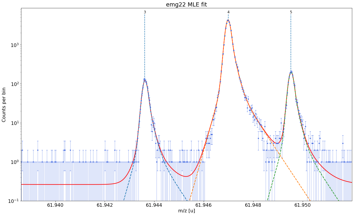
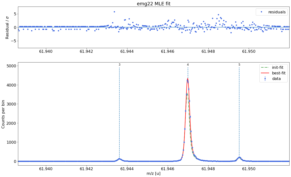
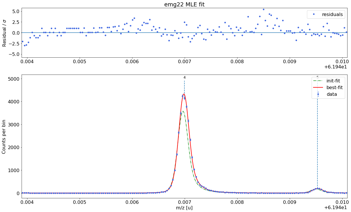
Plot the fit curve zoomed to a region of interest (optional)¶

For more detailed inspection of the fit, a zoom to peaks or regions of interest can be shown with the plot_fit_zoom method.

[8]:

spec.plot_fit_zoom(peak_indeces=[3,4]) # zoom to region around peaks 3 and 4

Export fit results¶

Once all peaks have been fitted, the results can be exported to an XLSX Excel file and a separate file with the peak-shape calibration parameters by using the save_results method. The XLSX file contains three sheets: 1. General properties the spectrum object, e.g. input filename, used version of emgfit and all relevant dependencies, …

2. The peak properties table and linear and logarithmic plots of the full spectrum fit. 3. The peak centroid shifts relative to the mass calibrant obtained in the peak-shape uncertainty evaluation.

[9]:

spec.save_results('outputs/'+filename+' fitting MLE')

ERROR: File outputs/2019-09-13_004-_006 SUMMED High stats 62Ga fitting MLE.xlsx already exists. No files saved! Choose a different filename or delete the original file and re-try.

That’s it! In principle we’re be done with the fitting at this point. Next we would probably take a look at the output file and proceed with some post-processing in Excel (e.g. combining mass values from different spectra etc.).

However, since emgfit gives the user a large amount of freedom, there’s are a number of things that could have been done differently depending on your preferences. So here is some possible…

Alternative procedures:¶

The above steps represent a full spectrum analysis. However, emgfit gives the user the freedom to take many different routes in processing the spectrum. Some of the possible alternatives are presented in the following:

Alternative 1: Performing the mass recalibration separately before the ion-of-interest fits¶

All steps up to the final peak fit are identical. For breviety here we simply create an exact clone of the above spectrum object:

[10]:

import copy
spec2 = copy.deepcopy(spec) # create a clone of the spectrum object

First obtain the recalibration factor from a fit of the mass calibrant¶

[11]:

spec2.fit_calibrant(species_mass_calib='Ti46:O16:-1e')

##### Calibrant fit #####

Model

((Model(constant, prefix='bkg_') + Model(emg22, prefix='p4_')) + Model(emg22, prefix='p5_'))

Fit Statistics

fitting method	least_squares
# function evals	9
# data points	169
# variables	5
chi-square	307.772018
reduced chi-square	1.87665864
Akaike info crit.	111.308840
Bayesian info crit.	126.958333

Variables

name	value	standard error	relative error	initial value	min	max	vary	expression
bkg_c	1.05752689	0.13337284	(12.61%)	0.1	0.00000000	4.00000000	True
p4_amp	1.24572232	0.00678229	(0.54%)	1.0294480000000001	1.0000e-20	inf	True
p4_mu	61.9470122	6.7237e-07	(0.00%)	61.946994300285866	61.9369943	61.9569943	True
p4_sigma	8.3298e-05	0.00000000	(0.00%)	8.329830944305415e-05	0.00000000	0.00508330	False
p4_theta	0.72958107	0.00000000	(0.00%)	0.7295810682165222	0.00000000	1.00000000	False
p4_eta_m1	0.93085594	0.00000000	(0.00%)	0.9308559436145877	0.00000000	1.00000000	False
p4_eta_m2	0.06914406	0.00000000	(0.00%)	0.06914405638541232	0.00000000	1.00000000	False	1-p4_eta_m1
p4_tau_m1	4.6426e-05	0.00000000	(0.00%)	4.6426492114914925e-05	1.0000e-12	0.05000000	False
p4_tau_m2	1.9392e-04	0.00000000	(0.00%)	0.0001939165239395595	1.0000e-12	0.05000000	False
p4_eta_p1	0.81292600	0.00000000	(0.00%)	0.8129260035354914	0.00000000	1.00000000	False
p4_eta_p2	0.18707400	0.00000000	(0.00%)	0.18707399646450862	0.00000000	1.00000000	False	1-p4_eta_p1
p4_tau_p1	1.2908e-04	0.00000000	(0.00%)	0.0001290811175724487	1.0000e-12	0.05000000	False
p4_tau_p2	4.5400e-04	0.00000000	(0.00%)	0.0004539974092137846	1.0000e-12	0.05000000	False
p5_amp	0.05637666	0.00148134	(2.63%)	0.050095999999999995	1.0000e-20	inf	True
p5_mu	61.9495591	3.2791e-06	(0.00%)	61.94952680789496	61.9395268	61.9595268	True
p5_sigma	8.3298e-05	0.00000000	(0.00%)	8.329830944305415e-05	0.00000000	0.00508330	False
p5_theta	0.72958107	0.00000000	(0.00%)	0.7295810682165222	0.00000000	1.00000000	False
p5_eta_m1	0.93085594	0.00000000	(0.00%)	0.9308559436145877	0.00000000	1.00000000	False
p5_eta_m2	0.06914406	0.00000000	(0.00%)	0.06914405638541232	0.00000000	1.00000000	False	1-p5_eta_m1
p5_tau_m1	4.6426e-05	0.00000000	(0.00%)	4.6426492114914925e-05	1.0000e-12	0.05000000	False
p5_tau_m2	1.9392e-04	0.00000000	(0.00%)	0.0001939165239395595	1.0000e-12	0.05000000	False
p5_eta_p1	0.81292600	0.00000000	(0.00%)	0.8129260035354914	0.00000000	1.00000000	False
p5_eta_p2	0.18707400	0.00000000	(0.00%)	0.18707399646450862	0.00000000	1.00000000	False	1-p5_eta_p1
p5_tau_p1	1.2908e-04	0.00000000	(0.00%)	0.0001290811175724487	1.0000e-12	0.05000000	False
p5_tau_p2	4.5400e-04	0.00000000	(0.00%)	0.0004539974092137846	1.0000e-12	0.05000000	False


##### Mass recalibration #####


Relative literature error of mass calibrant:    3e-09
Relative statistical error of mass calibrant:   1.2e-08

Recalibration factor:      0.999999689 = 1 -3.11e-07
Relative recalibration error:  1.2e-08

Determining absolute centroid shifts of mass calibrant.

Fit all peaks and use the mass recalibration factor from above to calculate the final mass values¶

[12]:

spec2.fit_peaks()


##### Peak-shape uncertainty evaluation #####

All mass shifts below are corrected for the corresponding shifts of the calibrant peak.

Determining absolute centroid shifts of mass calibrant.

Re-fitting with sigma = 8.33e-05 +/- 2.73e-06 shifts peak 0 by -0.200 /  0.184 μu.
Re-fitting with sigma = 8.33e-05 +/- 2.73e-06 shifts peak 1 by  0.469 / -0.391 μu.
Re-fitting with sigma = 8.33e-05 +/- 2.73e-06 shifts peak 2 by -0.371 /  0.232 μu.
Re-fitting with sigma = 8.33e-05 +/- 2.73e-06 shifts peak 3 by -0.021 /  0.026 μu.
Re-fitting with sigma = 8.33e-05 +/- 2.73e-06 shifts peak 5 by  0.032 / -0.069 μu.
Re-fitting with sigma = 8.33e-05 +/- 2.73e-06 shifts peak 6 by  0.052 / -0.003 μu.
Re-fitting with sigma = 8.33e-05 +/- 2.73e-06 shifts peak 7 by  0.228 / -0.189 μu.

Re-fitting with theta = 7.30e-01 +/- 2.08e-02 shifts peak 0 by -0.443 /  0.407 μu.
Re-fitting with theta = 7.30e-01 +/- 2.08e-02 shifts peak 1 by -0.897 /  0.948 μu.
Re-fitting with theta = 7.30e-01 +/- 2.08e-02 shifts peak 2 by -0.427 /  0.239 μu.
Re-fitting with theta = 7.30e-01 +/- 2.08e-02 shifts peak 3 by -0.148 /  0.158 μu.
Re-fitting with theta = 7.30e-01 +/- 2.08e-02 shifts peak 5 by -0.152 /  0.266 μu.
Re-fitting with theta = 7.30e-01 +/- 2.08e-02 shifts peak 6 by -0.081 /  0.084 μu.
Re-fitting with theta = 7.30e-01 +/- 2.08e-02 shifts peak 7 by -1.583 /  1.728 μu.

Re-fitting with eta_m1 = 9.31e-01 +/- 1.78e-02 shifts peak 0 by  0.534 / -0.505 μu.
Re-fitting with eta_m1 = 9.31e-01 +/- 1.78e-02 shifts peak 1 by  0.322 / -0.226 μu.
Re-fitting with eta_m1 = 9.31e-01 +/- 1.78e-02 shifts peak 2 by  0.228 / -0.418 μu.
Re-fitting with eta_m1 = 9.31e-01 +/- 1.78e-02 shifts peak 3 by  0.286 / -0.194 μu.
Re-fitting with eta_m1 = 9.31e-01 +/- 1.78e-02 shifts peak 5 by  0.244 / -0.155 μu.
Re-fitting with eta_m1 = 9.31e-01 +/- 1.78e-02 shifts peak 6 by  0.086 / -0.049 μu.
Re-fitting with eta_m1 = 9.31e-01 +/- 1.78e-02 shifts peak 7 by  0.460 / -0.330 μu.

Re-fitting with tau_m1 = 4.64e-05 +/- 5.07e-06 shifts peak 0 by -0.682 /  0.715 μu.
Re-fitting with tau_m1 = 4.64e-05 +/- 5.07e-06 shifts peak 1 by  0.226 / -0.195 μu.
Re-fitting with tau_m1 = 4.64e-05 +/- 5.07e-06 shifts peak 2 by -0.501 /  0.369 μu.
Re-fitting with tau_m1 = 4.64e-05 +/- 5.07e-06 shifts peak 3 by -0.070 /  0.151 μu.
Re-fitting with tau_m1 = 4.64e-05 +/- 5.07e-06 shifts peak 5 by -0.125 /  0.098 μu.
Re-fitting with tau_m1 = 4.64e-05 +/- 5.07e-06 shifts peak 6 by -0.030 / -0.021 μu.
Re-fitting with tau_m1 = 4.64e-05 +/- 5.07e-06 shifts peak 7 by -0.724 /  0.721 μu.

Re-fitting with tau_m2 = 1.94e-04 +/- 2.55e-05 shifts peak 0 by -0.241 /  0.260 μu.
Re-fitting with tau_m2 = 1.94e-04 +/- 2.55e-05 shifts peak 1 by -0.134 /  0.139 μu.
Re-fitting with tau_m2 = 1.94e-04 +/- 2.55e-05 shifts peak 2 by -0.254 /  0.043 μu.
Re-fitting with tau_m2 = 1.94e-04 +/- 2.55e-05 shifts peak 3 by -0.116 /  0.206 μu.
Re-fitting with tau_m2 = 1.94e-04 +/- 2.55e-05 shifts peak 5 by -0.048 /  0.171 μu.
Re-fitting with tau_m2 = 1.94e-04 +/- 2.55e-05 shifts peak 6 by -0.029 /  0.068 μu.
Re-fitting with tau_m2 = 1.94e-04 +/- 2.55e-05 shifts peak 7 by  0.215 / -0.015 μu.

Re-fitting with eta_p1 = 8.13e-01 +/- 3.62e-02 shifts peak 0 by -0.029 / -0.017 μu.
Re-fitting with eta_p1 = 8.13e-01 +/- 3.62e-02 shifts peak 1 by -0.194 /  0.103 μu.
Re-fitting with eta_p1 = 8.13e-01 +/- 3.62e-02 shifts peak 2 by -0.150 / -0.023 μu.
Re-fitting with eta_p1 = 8.13e-01 +/- 3.62e-02 shifts peak 3 by -0.086 /  0.088 μu.
Re-fitting with eta_p1 = 8.13e-01 +/- 3.62e-02 shifts peak 5 by -0.207 /  0.195 μu.
Re-fitting with eta_p1 = 8.13e-01 +/- 3.62e-02 shifts peak 6 by  0.043 /  0.003 μu.
Re-fitting with eta_p1 = 8.13e-01 +/- 3.62e-02 shifts peak 7 by -3.030 /  2.429 μu.

Re-fitting with tau_p1 = 1.29e-04 +/- 1.18e-05 shifts peak 0 by  0.020 / -0.125 μu.
Re-fitting with tau_p1 = 1.29e-04 +/- 1.18e-05 shifts peak 1 by  0.245 / -0.349 μu.
Re-fitting with tau_p1 = 1.29e-04 +/- 1.18e-05 shifts peak 2 by  0.191 / -0.497 μu.
Re-fitting with tau_p1 = 1.29e-04 +/- 1.18e-05 shifts peak 3 by  0.145 / -0.177 μu.
Re-fitting with tau_p1 = 1.29e-04 +/- 1.18e-05 shifts peak 5 by  0.042 /  0.007 μu.
Re-fitting with tau_p1 = 1.29e-04 +/- 1.18e-05 shifts peak 6 by -0.008 /  0.014 μu.
Re-fitting with tau_p1 = 1.29e-04 +/- 1.18e-05 shifts peak 7 by  0.444 / -0.461 μu.

Re-fitting with tau_p2 = 4.54e-04 +/- 5.93e-05 shifts peak 0 by -0.066 /  0.074 μu.
Re-fitting with tau_p2 = 4.54e-04 +/- 5.93e-05 shifts peak 1 by  0.330 / -0.326 μu.
Re-fitting with tau_p2 = 4.54e-04 +/- 5.93e-05 shifts peak 2 by  0.024 / -0.020 μu.
Re-fitting with tau_p2 = 4.54e-04 +/- 5.93e-05 shifts peak 3 by  0.039 / -0.026 μu.
Re-fitting with tau_p2 = 4.54e-04 +/- 5.93e-05 shifts peak 5 by  0.382 / -0.444 μu.
Re-fitting with tau_p2 = 4.54e-04 +/- 5.93e-05 shifts peak 6 by -0.026 /  0.046 μu.
Re-fitting with tau_p2 = 4.54e-04 +/- 5.93e-05 shifts peak 7 by  1.375 / -6.324 μu.

Relative peak-shape error of peak 0: 1.7e-08
Relative peak-shape error of peak 1: 2e-08
Relative peak-shape error of peak 2: 1.7e-08
Relative peak-shape error of peak 3: 7e-09
Relative peak-shape error of peak 5: 1e-08
Relative peak-shape error of peak 6: 3e-09
Relative peak-shape error of peak 7: 1.18e-07

	x_pos	species	comment	m_AME	m_AME_error	extrapolated	fit_model	cost_func	red_chi	area	area_error	m_ion	rel_stat_error	rel_recal_error	rel_peakshape_error	rel_mass_error	A	atomic_ME_keV	mass_error_keV	m_dev_keV
0	61.927800	Ni62:-1e	-	61.927796	4.700000e-07	False	emg22	MLE	1.22	38.67	6.77	61.927795	3.443261e-07	1.196007e-08	1.711439e-08	3.449586e-07	62.0	-66747.125	19.899064	-0.795
1	61.932021	Cu62:-1e?	-	NaN	NaN	False	emg22	MLE	1.22	28.07	5.98	61.932051	4.041159e-07	1.196007e-08	2.017659e-08	4.047960e-07	NaN	NaN	23.352415	NaN
2	61.934369	?	Non-isobaric	NaN	NaN	False	emg22	MLE	1.22	3872.82	62.56	61.934369	3.440307e-08	1.196007e-08	1.678810e-08	4.010555e-08	NaN	NaN	2.313749	NaN
3	61.943618	Ga62:-1e	-	61.943641	6.940000e-07	False	emg22	MLE	1.22	954.58	31.20	61.943636	6.928509e-08	1.196007e-08	7.461555e-09	7.070461e-08	62.0	-51992.065	4.079665	-5.153
4	61.946994	Ti46:O16:-1e	mass calibrant	61.946993	1.760001e-07	False	emg22	MLE	1.88	33947.16	184.82	61.946993	1.161771e-08	1.196007e-08	NaN	NaN	62.0	-48864.806	NaN	0.000
5	61.949527	Sc46:O16:-1e	-	61.949534	7.320000e-07	False	emg22	MLE	1.22	1567.77	40.11	61.949540	5.405842e-08	1.196007e-08	1.048731e-08	5.635016e-08	62.0	-46492.223	3.251721	6.002
6	61.956611	Ca43:F19:-1e	shape calibrant	61.956621	2.440018e-07	False	emg22	MLE	1.22	25966.02	161.32	61.956622	1.328166e-08	1.196007e-08	2.639493e-09	1.806689e-08	62.0	-39895.693	1.042681	0.578
7	61.958997	?	-	NaN	NaN	False	emg22	MLE	1.22	25.28	6.40	61.959019	4.256470e-07	1.196007e-08	1.177199e-07	4.417877e-07	NaN	NaN	25.497540	NaN

The values for chi-squared as well as the parameter uncertainties and correlations reported by lmfit below should be taken with caution when your MLE fit includes bins with low statistics. For details see Notes section in the spectrum.peakfit() method documentation.

Model

((((((((Model(constant, prefix='bkg_') + Model(emg22, prefix='p0_')) + Model(emg22, prefix='p1_')) + Model(emg22, prefix='p2_')) + Model(emg22, prefix='p3_')) + Model(emg22, prefix='p4_')) + Model(emg22, prefix='p5_')) + Model(emg22, prefix='p6_')) + Model(emg22, prefix='p7_'))

Fit Statistics

fitting method	least_squares
# function evals	9
# data points	1027
# variables	17
chi-square	1237.06416
reduced chi-square	1.22481600
Akaike info crit.	225.123700
Bayesian info crit.	309.008452

Variables

name	value	standard error	relative error	initial value	min	max	vary	expression
bkg_c	0.26119680	0.02315482	(8.86%)	0.1	0.00000000	4.00000000	True
p0_amp	0.00141907	2.4842e-04	(17.51%)	0.001488	1.0000e-20	inf	True
p0_mu	61.9278147	2.2955e-05	(0.00%)	61.927800309876424	61.9178003	61.9378003	True
p0_sigma	8.3298e-05	0.00000000	(0.00%)	8.329830944305415e-05	0.00000000	0.00508330	False
p0_theta	0.72958107	0.00000000	(0.00%)	0.7295810682165222	0.00000000	1.00000000	False
p0_eta_m1	0.93085594	0.00000000	(0.00%)	0.9308559436145877	0.00000000	1.00000000	False
p0_eta_m2	0.06914406	0.00000000	(0.00%)	0.06914405638541232	0.00000000	1.00000000	False	1-p0_eta_m1
p0_tau_m1	4.6426e-05	0.00000000	(0.00%)	4.6426492114914925e-05	1.0000e-12	0.05000000	False
p0_tau_m2	1.9392e-04	0.00000000	(0.00%)	0.0001939165239395595	1.0000e-12	0.05000000	False
p0_eta_p1	0.81292600	0.00000000	(0.00%)	0.8129260035354914	0.00000000	1.00000000	False
p0_eta_p2	0.18707400	0.00000000	(0.00%)	0.18707399646450862	0.00000000	1.00000000	False	1-p0_eta_p1
p0_tau_p1	1.2908e-04	0.00000000	(0.00%)	0.0001290811175724487	1.0000e-12	0.05000000	False
p0_tau_p2	4.5400e-04	0.00000000	(0.00%)	0.0004539974092137846	1.0000e-12	0.05000000	False
p1_amp	0.00103012	2.1954e-04	(21.31%)	0.000496	1.0000e-20	inf	True
p1_mu	61.9320700	2.7212e-05	(0.00%)	61.93202053070152	61.9220205	61.9420205	True
p1_sigma	8.3298e-05	0.00000000	(0.00%)	8.329830944305415e-05	0.00000000	0.00508330	False
p1_theta	0.72958107	0.00000000	(0.00%)	0.7295810682165222	0.00000000	1.00000000	False
p1_eta_m1	0.93085594	0.00000000	(0.00%)	0.9308559436145877	0.00000000	1.00000000	False
p1_eta_m2	0.06914406	0.00000000	(0.00%)	0.06914405638541232	0.00000000	1.00000000	False	1-p1_eta_m1
p1_tau_m1	4.6426e-05	0.00000000	(0.00%)	4.6426492114914925e-05	1.0000e-12	0.05000000	False
p1_tau_m2	1.9392e-04	0.00000000	(0.00%)	0.0001939165239395595	1.0000e-12	0.05000000	False
p1_eta_p1	0.81292600	0.00000000	(0.00%)	0.8129260035354914	0.00000000	1.00000000	False
p1_eta_p2	0.18707400	0.00000000	(0.00%)	0.18707399646450862	0.00000000	1.00000000	False	1-p1_eta_p1
p1_tau_p1	1.2908e-04	0.00000000	(0.00%)	0.0001290811175724487	1.0000e-12	0.05000000	False
p1_tau_p2	4.5400e-04	0.00000000	(0.00%)	0.0004539974092137846	1.0000e-12	0.05000000	False
p2_amp	0.14211660	0.00229567	(1.62%)	0.15648800000000002	1.0000e-20	inf	True
p2_mu	61.9343887	2.0515e-06	(0.00%)	61.93436923761443	61.9243692	61.9443692	True
p2_sigma	8.3298e-05	0.00000000	(0.00%)	8.329830944305415e-05	0.00000000	0.00508330	False
p2_theta	0.72958107	0.00000000	(0.00%)	0.7295810682165222	0.00000000	1.00000000	False
p2_eta_m1	0.93085594	0.00000000	(0.00%)	0.9308559436145877	0.00000000	1.00000000	False
p2_eta_m2	0.06914406	0.00000000	(0.00%)	0.06914405638541232	0.00000000	1.00000000	False	1-p2_eta_m1
p2_tau_m1	4.6426e-05	0.00000000	(0.00%)	4.6426492114914925e-05	1.0000e-12	0.05000000	False
p2_tau_m2	1.9392e-04	0.00000000	(0.00%)	0.0001939165239395595	1.0000e-12	0.05000000	False
p2_eta_p1	0.81292600	0.00000000	(0.00%)	0.8129260035354914	0.00000000	1.00000000	False
p2_eta_p2	0.18707400	0.00000000	(0.00%)	0.18707399646450862	0.00000000	1.00000000	False	1-p2_eta_p1
p2_tau_p1	1.2908e-04	0.00000000	(0.00%)	0.0001290811175724487	1.0000e-12	0.05000000	False
p2_tau_p2	4.5400e-04	0.00000000	(0.00%)	0.0004539974092137846	1.0000e-12	0.05000000	False
p3_amp	0.03502903	0.00114480	(3.27%)	0.031992	1.0000e-20	inf	True
p3_mu	61.9436549	4.0836e-06	(0.00%)	61.943617703998214	61.9336177	61.9536177	True
p3_sigma	8.3298e-05	0.00000000	(0.00%)	8.329830944305415e-05	0.00000000	0.00508330	False
p3_theta	0.72958107	0.00000000	(0.00%)	0.7295810682165222	0.00000000	1.00000000	False
p3_eta_m1	0.93085594	0.00000000	(0.00%)	0.9308559436145877	0.00000000	1.00000000	False
p3_eta_m2	0.06914406	0.00000000	(0.00%)	0.06914405638541232	0.00000000	1.00000000	False	1-p3_eta_m1
p3_tau_m1	4.6426e-05	0.00000000	(0.00%)	4.6426492114914925e-05	1.0000e-12	0.05000000	False
p3_tau_m2	1.9392e-04	0.00000000	(0.00%)	0.0001939165239395595	1.0000e-12	0.05000000	False
p3_eta_p1	0.81292600	0.00000000	(0.00%)	0.8129260035354914	0.00000000	1.00000000	False
p3_eta_p2	0.18707400	0.00000000	(0.00%)	0.18707399646450862	0.00000000	1.00000000	False	1-p3_eta_p1
p3_tau_p1	1.2908e-04	0.00000000	(0.00%)	0.0001290811175724487	1.0000e-12	0.05000000	False
p3_tau_p2	4.5400e-04	0.00000000	(0.00%)	0.0004539974092137846	1.0000e-12	0.05000000	False
p4_amp	1.24782758	0.00684747	(0.55%)	1.0294480000000001	1.0000e-20	inf	True
p4_mu	61.9470121	6.8949e-07	(0.00%)	61.946994300285866	61.9369943	61.9569943	True
p4_sigma	8.3298e-05	0.00000000	(0.00%)	8.329830944305415e-05	0.00000000	0.00508330	False
p4_theta	0.72958107	0.00000000	(0.00%)	0.7295810682165222	0.00000000	1.00000000	False
p4_eta_m1	0.93085594	0.00000000	(0.00%)	0.9308559436145877	0.00000000	1.00000000	False
p4_eta_m2	0.06914406	0.00000000	(0.00%)	0.06914405638541232	0.00000000	1.00000000	False	1-p4_eta_m1
p4_tau_m1	4.6426e-05	0.00000000	(0.00%)	4.6426492114914925e-05	1.0000e-12	0.05000000	False
p4_tau_m2	1.9392e-04	0.00000000	(0.00%)	0.0001939165239395595	1.0000e-12	0.05000000	False
p4_eta_p1	0.81292600	0.00000000	(0.00%)	0.8129260035354914	0.00000000	1.00000000	False
p4_eta_p2	0.18707400	0.00000000	(0.00%)	0.18707399646450862	0.00000000	1.00000000	False	1-p4_eta_p1
p4_tau_p1	1.2908e-04	0.00000000	(0.00%)	0.0001290811175724487	1.0000e-12	0.05000000	False
p4_tau_p2	4.5400e-04	0.00000000	(0.00%)	0.0004539974092137846	1.0000e-12	0.05000000	False
p5_amp	0.05753078	0.00147176	(2.56%)	0.050095999999999995	1.0000e-20	inf	True
p5_mu	61.9495592	3.1967e-06	(0.00%)	61.94952680789496	61.9395268	61.9595268	True
p5_sigma	8.3298e-05	0.00000000	(0.00%)	8.329830944305415e-05	0.00000000	0.00508330	False
p5_theta	0.72958107	0.00000000	(0.00%)	0.7295810682165222	0.00000000	1.00000000	False
p5_eta_m1	0.93085594	0.00000000	(0.00%)	0.9308559436145877	0.00000000	1.00000000	False
p5_eta_m2	0.06914406	0.00000000	(0.00%)	0.06914405638541232	0.00000000	1.00000000	False	1-p5_eta_m1
p5_tau_m1	4.6426e-05	0.00000000	(0.00%)	4.6426492114914925e-05	1.0000e-12	0.05000000	False
p5_tau_m2	1.9392e-04	0.00000000	(0.00%)	0.0001939165239395595	1.0000e-12	0.05000000	False
p5_eta_p1	0.81292600	0.00000000	(0.00%)	0.8129260035354914	0.00000000	1.00000000	False
p5_eta_p2	0.18707400	0.00000000	(0.00%)	0.18707399646450862	0.00000000	1.00000000	False	1-p5_eta_p1
p5_tau_p1	1.2908e-04	0.00000000	(0.00%)	0.0001290811175724487	1.0000e-12	0.05000000	False
p5_tau_p2	4.5400e-04	0.00000000	(0.00%)	0.0004539974092137846	1.0000e-12	0.05000000	False
p6_amp	0.95284700	0.00591978	(0.62%)	0.8422080000000001	1.0000e-20	inf	True
p6_mu	61.9566409	7.7273e-07	(0.00%)	61.95661076349748	61.9466108	61.9666108	True
p6_sigma	8.3298e-05	0.00000000	(0.00%)	8.329830944305415e-05	0.00000000	0.00508330	False
p6_theta	0.72958107	0.00000000	(0.00%)	0.7295810682165222	0.00000000	1.00000000	False
p6_eta_m1	0.93085594	0.00000000	(0.00%)	0.9308559436145877	0.00000000	1.00000000	False
p6_eta_m2	0.06914406	0.00000000	(0.00%)	0.06914405638541232	0.00000000	1.00000000	False	1-p6_eta_m1
p6_tau_m1	4.6426e-05	0.00000000	(0.00%)	4.6426492114914925e-05	1.0000e-12	0.05000000	False
p6_tau_m2	1.9392e-04	0.00000000	(0.00%)	0.0001939165239395595	1.0000e-12	0.05000000	False
p6_eta_p1	0.81292600	0.00000000	(0.00%)	0.8129260035354914	0.00000000	1.00000000	False
p6_eta_p2	0.18707400	0.00000000	(0.00%)	0.18707399646450862	0.00000000	1.00000000	False	1-p6_eta_p1
p6_tau_p1	1.2908e-04	0.00000000	(0.00%)	0.0001290811175724487	1.0000e-12	0.05000000	False
p6_tau_p2	4.5400e-04	0.00000000	(0.00%)	0.0004539974092137846	1.0000e-12	0.05000000	False
p7_amp	9.2777e-04	2.3485e-04	(25.31%)	0.001488	1.0000e-20	inf	True
p7_mu	61.9590381	3.6728e-05	(0.00%)	61.95899664282278	61.9489966	61.9689966	True
p7_sigma	8.3298e-05	0.00000000	(0.00%)	8.329830944305415e-05	0.00000000	0.00508330	False
p7_theta	0.72958107	0.00000000	(0.00%)	0.7295810682165222	0.00000000	1.00000000	False
p7_eta_m1	0.93085594	0.00000000	(0.00%)	0.9308559436145877	0.00000000	1.00000000	False
p7_eta_m2	0.06914406	0.00000000	(0.00%)	0.06914405638541232	0.00000000	1.00000000	False	1-p7_eta_m1
p7_tau_m1	4.6426e-05	0.00000000	(0.00%)	4.6426492114914925e-05	1.0000e-12	0.05000000	False
p7_tau_m2	1.9392e-04	0.00000000	(0.00%)	0.0001939165239395595	1.0000e-12	0.05000000	False
p7_eta_p1	0.81292600	0.00000000	(0.00%)	0.8129260035354914	0.00000000	1.00000000	False
p7_eta_p2	0.18707400	0.00000000	(0.00%)	0.18707399646450862	0.00000000	1.00000000	False	1-p7_eta_p1
p7_tau_p1	1.2908e-04	0.00000000	(0.00%)	0.0001290811175724487	1.0000e-12	0.05000000	False
p7_tau_p2	4.5400e-04	0.00000000	(0.00%)	0.0004539974092137846	1.0000e-12	0.05000000	False

Correlations (unreported correlations are < 0.100)

p4_amp	p4_mu	-0.1469
p7_amp	p7_mu	-0.1139

Alternative 2: Chi-square instead of MLE fitting¶

All steps up to the final peak fit are identical. For breviety here we simply create an exact clone of the above spectrum object and re-use the above peak-shape calibration (obtained with chi-square fitting):

[13]:

import copy
spec_chi_sq = copy.deepcopy(spec) # create a clone of the spectrum object

# Use Pearson's chi-squared statistic for A_stat_emg determination
spec_chi_sq.determine_A_stat_emg(species='Ca43:F19:-1e',x_range=0.004,cost_func='chi-square',plot_filename='outputs/'+filename+'_chi-square',N_spectra=10)

Creating synthetic spectra via bootstrap re-sampling and fitting  them for A_stat determination.
Depending on the choice of `N_spectra` this can take a few minutes. Interrupt kernel if this takes too long.


Done!

[[Model]]
    Model(powerlaw)
[[Fit Statistics]]
    # fitting method   = leastsq
    # function evals   = 5
    # data points      = 8
    # variables        = 1
    chi-square         = 8.9947e-09
    reduced chi-square = 1.2850e-09
    Akaike info crit   = -162.848615
    Bayesian info crit = -162.769174
[[Variables]]
    amplitude:  1.4857e-04 +/- 1.2998e-05 (8.75%) (init = 1)
    exponent:  -0.5 (fixed)

A_stat of a Gaussian model: 0.425
Default A_stat_emg for Hyper-EMG models: 0.52
A_stat_emg for this spectrum's emg22 fit model: 0.619 +- 0.054

[14]:

spec_chi_sq.fit_peaks(species_mass_calib='Ti46:O16:-1e',cost_func='chi-square') # use Pearson's chi-squared statistic


##### Mass recalibration #####


Relative literature error of mass calibrant:    3e-09
Relative statistical error of mass calibrant:   1.3e-08

Recalibration factor:      0.999999689 = 1 -3.11e-07
Relative recalibration error:  1.3e-08


##### Peak-shape uncertainty evaluation #####

All mass shifts below are corrected for the corresponding shifts of the calibrant peak.

Determining absolute centroid shifts of mass calibrant.

Re-fitting with sigma = 8.33e-05 +/- 2.73e-06 shifts peak 0 by -2.553 / -0.335 μu.
Re-fitting with sigma = 8.33e-05 +/- 2.73e-06 shifts peak 1 by -0.135 /  0.066 μu.
Re-fitting with sigma = 8.33e-05 +/- 2.73e-06 shifts peak 2 by -0.384 /  0.272 μu.
Re-fitting with sigma = 8.33e-05 +/- 2.73e-06 shifts peak 3 by -0.092 /  0.077 μu.
Re-fitting with sigma = 8.33e-05 +/- 2.73e-06 shifts peak 5 by -0.028 /  0.030 μu.
Re-fitting with sigma = 8.33e-05 +/- 2.73e-06 shifts peak 6 by  0.010 / -0.011 μu.
Re-fitting with sigma = 8.33e-05 +/- 2.73e-06 shifts peak 7 by -0.678 /  1.590 μu.

Re-fitting with theta = 7.30e-01 +/- 2.08e-02 shifts peak 0 by -0.907 /  0.870 μu.
Re-fitting with theta = 7.30e-01 +/- 2.08e-02 shifts peak 1 by -0.928 /  0.734 μu.
Re-fitting with theta = 7.30e-01 +/- 2.08e-02 shifts peak 2 by -0.665 /  0.527 μu.
Re-fitting with theta = 7.30e-01 +/- 2.08e-02 shifts peak 3 by -0.203 /  0.180 μu.
Re-fitting with theta = 7.30e-01 +/- 2.08e-02 shifts peak 5 by -0.143 /  0.145 μu.
Re-fitting with theta = 7.30e-01 +/- 2.08e-02 shifts peak 6 by -0.015 /  0.018 μu.
Re-fitting with theta = 7.30e-01 +/- 2.08e-02 shifts peak 7 by -1.595 /  2.653 μu.

Re-fitting with eta_m1 = 9.31e-01 +/- 1.78e-02 shifts peak 0 by  0.620 / -0.475 μu.
Re-fitting with eta_m1 = 9.31e-01 +/- 1.78e-02 shifts peak 1 by  0.548 / -0.406 μu.
Re-fitting with eta_m1 = 9.31e-01 +/- 1.78e-02 shifts peak 2 by  0.342 / -0.302 μu.
Re-fitting with eta_m1 = 9.31e-01 +/- 1.78e-02 shifts peak 3 by  0.323 / -0.225 μu.
Re-fitting with eta_m1 = 9.31e-01 +/- 1.78e-02 shifts peak 5 by  0.176 / -0.107 μu.
Re-fitting with eta_m1 = 9.31e-01 +/- 1.78e-02 shifts peak 6 by  0.018 / -0.015 μu.
Re-fitting with eta_m1 = 9.31e-01 +/- 1.78e-02 shifts peak 7 by  0.628 / -0.509 μu.

Re-fitting with tau_m1 = 4.64e-05 +/- 5.07e-06 shifts peak 0 by -3.304 /  0.435 μu.
Re-fitting with tau_m1 = 4.64e-05 +/- 5.07e-06 shifts peak 1 by -0.120 /  0.196 μu.
Re-fitting with tau_m1 = 4.64e-05 +/- 5.07e-06 shifts peak 2 by -0.486 /  0.505 μu.
Re-fitting with tau_m1 = 4.64e-05 +/- 5.07e-06 shifts peak 3 by -0.226 /  0.224 μu.
Re-fitting with tau_m1 = 4.64e-05 +/- 5.07e-06 shifts peak 5 by -0.216 /  0.217 μu.
Re-fitting with tau_m1 = 4.64e-05 +/- 5.07e-06 shifts peak 6 by -0.033 /  0.031 μu.
Re-fitting with tau_m1 = 4.64e-05 +/- 5.07e-06 shifts peak 7 by -1.950 /  2.106 μu.

Re-fitting with tau_m2 = 1.94e-04 +/- 2.55e-05 shifts peak 0 by -0.121 /  0.244 μu.
Re-fitting with tau_m2 = 1.94e-04 +/- 2.55e-05 shifts peak 1 by -0.268 /  0.340 μu.
Re-fitting with tau_m2 = 1.94e-04 +/- 2.55e-05 shifts peak 2 by -0.061 /  0.105 μu.
Re-fitting with tau_m2 = 1.94e-04 +/- 2.55e-05 shifts peak 3 by -0.093 /  0.171 μu.
Re-fitting with tau_m2 = 1.94e-04 +/- 2.55e-05 shifts peak 5 by  0.006 /  0.048 μu.
Re-fitting with tau_m2 = 1.94e-04 +/- 2.55e-05 shifts peak 6 by  0.016 / -0.008 μu.
Re-fitting with tau_m2 = 1.94e-04 +/- 2.55e-05 shifts peak 7 by -0.120 /  0.174 μu.

Re-fitting with eta_p1 = 8.13e-01 +/- 3.62e-02 shifts peak 0 by -0.143 /  0.069 μu.
Re-fitting with eta_p1 = 8.13e-01 +/- 3.62e-02 shifts peak 1 by -0.309 /  0.132 μu.
Re-fitting with eta_p1 = 8.13e-01 +/- 3.62e-02 shifts peak 2 by -0.327 /  0.191 μu.
Re-fitting with eta_p1 = 8.13e-01 +/- 3.62e-02 shifts peak 3 by -0.136 /  0.112 μu.
Re-fitting with eta_p1 = 8.13e-01 +/- 3.62e-02 shifts peak 5 by -0.229 /  0.207 μu.
Re-fitting with eta_p1 = 8.13e-01 +/- 3.62e-02 shifts peak 6 by  0.018 / -0.015 μu.
Re-fitting with eta_p1 = 8.13e-01 +/- 3.62e-02 shifts peak 7 by -8.185 /  6.416 μu.

Re-fitting with tau_p1 = 1.29e-04 +/- 1.18e-05 shifts peak 0 by  0.153 / -0.285 μu.
Re-fitting with tau_p1 = 1.29e-04 +/- 1.18e-05 shifts peak 1 by  0.517 / -0.704 μu.
Re-fitting with tau_p1 = 1.29e-04 +/- 1.18e-05 shifts peak 2 by  0.487 / -0.596 μu.
Re-fitting with tau_p1 = 1.29e-04 +/- 1.18e-05 shifts peak 3 by  0.168 / -0.207 μu.
Re-fitting with tau_p1 = 1.29e-04 +/- 1.18e-05 shifts peak 5 by -0.072 /  0.074 μu.
Re-fitting with tau_p1 = 1.29e-04 +/- 1.18e-05 shifts peak 6 by -0.002 /  0.000 μu.
Re-fitting with tau_p1 = 1.29e-04 +/- 1.18e-05 shifts peak 7 by  0.045 / -0.070 μu.

Re-fitting with tau_p2 = 4.54e-04 +/- 5.93e-05 shifts peak 0 by  0.011 / -2.820 μu.
Re-fitting with tau_p2 = 4.54e-04 +/- 5.93e-05 shifts peak 1 by -0.050 / -0.131 μu.
Re-fitting with tau_p2 = 4.54e-04 +/- 5.93e-05 shifts peak 2 by -0.011 / -0.139 μu.
Re-fitting with tau_p2 = 4.54e-04 +/- 5.93e-05 shifts peak 3 by  0.021 / -0.066 μu.
Re-fitting with tau_p2 = 4.54e-04 +/- 5.93e-05 shifts peak 5 by  0.476 / -0.625 μu.
Re-fitting with tau_p2 = 4.54e-04 +/- 5.93e-05 shifts peak 6 by -0.018 /  0.024 μu.
Re-fitting with tau_p2 = 4.54e-04 +/- 5.93e-05 shifts peak 7 by  8.496 / -29.021 μu.

Relative peak-shape error of peak 0: 8.4e-08
Relative peak-shape error of peak 1: 2.3e-08
Relative peak-shape error of peak 2: 1.9e-08
Relative peak-shape error of peak 3: 9e-09
Relative peak-shape error of peak 5: 1.2e-08
Relative peak-shape error of peak 6: 1e-09
Relative peak-shape error of peak 7: 4.91e-07

	x_pos	species	comment	m_AME	m_AME_error	extrapolated	fit_model	cost_func	red_chi	area	area_error	m_ion	rel_stat_error	rel_recal_error	rel_peakshape_error	rel_mass_error	A	atomic_ME_keV	mass_error_keV	m_dev_keV
0	61.927800	Ni62:-1e	-	61.927796	4.700000e-07	False	emg22	chi-square	0.78	42.98	7.29	61.927802	3.659375e-07	1.330349e-08	8.351916e-08	3.755832e-07	62.0	-66741.279	21.665659	5.051
1	61.932021	Cu62:-1e?	-	NaN	NaN	False	emg22	chi-square	0.78	31.37	6.53	61.932058	4.283049e-07	1.330349e-08	2.250747e-08	4.291022e-07	NaN	NaN	24.754625	NaN
2	61.934369	?	Non-isobaric	NaN	NaN	False	emg22	chi-square	0.78	4002.37	63.93	61.934370	3.791713e-08	1.330349e-08	1.946335e-08	4.464878e-08	NaN	NaN	2.575855	NaN
3	61.943618	Ga62:-1e	-	61.943641	6.940000e-07	False	emg22	chi-square	0.78	967.82	31.50	61.943636	7.709600e-08	1.330349e-08	8.848839e-09	7.873423e-08	62.0	-51992.161	4.542975	-5.248
4	61.946994	Ti46:O16:-1e	mass calibrant	61.946993	1.760001e-07	False	emg22	chi-square	0.78	34052.89	184.77	61.946993	1.299656e-08	1.330349e-08	NaN	NaN	62.0	-48864.806	NaN	0.000
5	61.949527	Sc46:O16:-1e	-	61.949534	7.320000e-07	False	emg22	chi-square	0.78	1582.90	40.49	61.949540	6.027830e-08	1.330349e-08	1.198125e-08	6.288090e-08	62.0	-46492.156	3.628582	6.070
6	61.956611	Ca43:F19:-1e	shape calibrant	61.956621	2.440018e-07	False	emg22	chi-square	0.78	26004.76	161.51	61.956622	1.487002e-08	1.330349e-08	8.904345e-10	1.997231e-08	62.0	-39895.706	1.152647	0.565
7	61.958997	?	-	NaN	NaN	False	emg22	chi-square	0.78	29.96	7.06	61.959002	4.380771e-07	1.330349e-08	4.905103e-07	6.577909e-07	NaN	NaN	37.964036	NaN

Model

((((((((Model(constant, prefix='bkg_') + Model(emg22, prefix='p0_')) + Model(emg22, prefix='p1_')) + Model(emg22, prefix='p2_')) + Model(emg22, prefix='p3_')) + Model(emg22, prefix='p4_')) + Model(emg22, prefix='p5_')) + Model(emg22, prefix='p6_')) + Model(emg22, prefix='p7_'))

Fit Statistics

fitting method	least_squares
# function evals	7
# data points	1027
# variables	17
chi-square	789.027165
reduced chi-square	0.78121502
Akaike info crit.	-236.713564
Bayesian info crit.	-152.828811

Variables

name	value	standard error	relative error	initial value	min	max	vary	expression
bkg_c	0.26881088	0.03720715	(13.84%)	0.1	0.00000000	4.00000000	True
p0_amp	0.00157708	2.6752e-04	(16.96%)	0.001488	1.0000e-20	inf	True
p0_mu	61.9278210	2.3311e-05	(0.00%)	61.927800309876424	61.9178003	61.9378003	True
p0_sigma	8.3298e-05	0.00000000	(0.00%)	8.329830944305415e-05	0.00000000	0.00508330	False
p0_theta	0.72958107	0.00000000	(0.00%)	0.7295810682165222	0.00000000	1.00000000	False
p0_eta_m1	0.93085594	0.00000000	(0.00%)	0.9308559436145877	0.00000000	1.00000000	False
p0_eta_m2	0.06914406	0.00000000	(0.00%)	0.06914405638541232	0.00000000	1.00000000	False	1-p0_eta_m1
p0_tau_m1	4.6426e-05	0.00000000	(0.00%)	4.6426492114914925e-05	1.0000e-12	0.05000000	False
p0_tau_m2	1.9392e-04	0.00000000	(0.00%)	0.0001939165239395595	1.0000e-12	0.05000000	False
p0_eta_p1	0.81292600	0.00000000	(0.00%)	0.8129260035354914	0.00000000	1.00000000	False
p0_eta_p2	0.18707400	0.00000000	(0.00%)	0.18707399646450862	0.00000000	1.00000000	False	1-p0_eta_p1
p0_tau_p1	1.2908e-04	0.00000000	(0.00%)	0.0001290811175724487	1.0000e-12	0.05000000	False
p0_tau_p2	4.5400e-04	0.00000000	(0.00%)	0.0004539974092137846	1.0000e-12	0.05000000	False
p1_amp	0.00115121	2.3959e-04	(20.81%)	0.000496	1.0000e-20	inf	True
p1_mu	61.9320777	2.5981e-05	(0.00%)	61.93202053070152	61.9220205	61.9420205	True
p1_sigma	8.3298e-05	0.00000000	(0.00%)	8.329830944305415e-05	0.00000000	0.00508330	False
p1_theta	0.72958107	0.00000000	(0.00%)	0.7295810682165222	0.00000000	1.00000000	False
p1_eta_m1	0.93085594	0.00000000	(0.00%)	0.9308559436145877	0.00000000	1.00000000	False
p1_eta_m2	0.06914406	0.00000000	(0.00%)	0.06914405638541232	0.00000000	1.00000000	False	1-p1_eta_m1
p1_tau_m1	4.6426e-05	0.00000000	(0.00%)	4.6426492114914925e-05	1.0000e-12	0.05000000	False
p1_tau_m2	1.9392e-04	0.00000000	(0.00%)	0.0001939165239395595	1.0000e-12	0.05000000	False
p1_eta_p1	0.81292600	0.00000000	(0.00%)	0.8129260035354914	0.00000000	1.00000000	False
p1_eta_p2	0.18707400	0.00000000	(0.00%)	0.18707399646450862	0.00000000	1.00000000	False	1-p1_eta_p1
p1_tau_p1	1.2908e-04	0.00000000	(0.00%)	0.0001290811175724487	1.0000e-12	0.05000000	False
p1_tau_p2	4.5400e-04	0.00000000	(0.00%)	0.0004539974092137846	1.0000e-12	0.05000000	False
p2_amp	0.14687054	0.00234596	(1.60%)	0.15648800000000002	1.0000e-20	inf	True
p2_mu	61.9343894	2.1344e-06	(0.00%)	61.93436923761443	61.9243692	61.9443692	True
p2_sigma	8.3298e-05	0.00000000	(0.00%)	8.329830944305415e-05	0.00000000	0.00508330	False
p2_theta	0.72958107	0.00000000	(0.00%)	0.7295810682165222	0.00000000	1.00000000	False
p2_eta_m1	0.93085594	0.00000000	(0.00%)	0.9308559436145877	0.00000000	1.00000000	False
p2_eta_m2	0.06914406	0.00000000	(0.00%)	0.06914405638541232	0.00000000	1.00000000	False	1-p2_eta_m1
p2_tau_m1	4.6426e-05	0.00000000	(0.00%)	4.6426492114914925e-05	1.0000e-12	0.05000000	False
p2_tau_m2	1.9392e-04	0.00000000	(0.00%)	0.0001939165239395595	1.0000e-12	0.05000000	False
p2_eta_p1	0.81292600	0.00000000	(0.00%)	0.8129260035354914	0.00000000	1.00000000	False
p2_eta_p2	0.18707400	0.00000000	(0.00%)	0.18707399646450862	0.00000000	1.00000000	False	1-p2_eta_p1
p2_tau_p1	1.2908e-04	0.00000000	(0.00%)	0.0001290811175724487	1.0000e-12	0.05000000	False
p2_tau_p2	4.5400e-04	0.00000000	(0.00%)	0.0004539974092137846	1.0000e-12	0.05000000	False
p3_amp	0.03551501	0.00115594	(3.25%)	0.031992	1.0000e-20	inf	True
p3_mu	61.9436548	4.0941e-06	(0.00%)	61.943617703998214	61.9336177	61.9536177	True
p3_sigma	8.3298e-05	0.00000000	(0.00%)	8.329830944305415e-05	0.00000000	0.00508330	False
p3_theta	0.72958107	0.00000000	(0.00%)	0.7295810682165222	0.00000000	1.00000000	False
p3_eta_m1	0.93085594	0.00000000	(0.00%)	0.9308559436145877	0.00000000	1.00000000	False
p3_eta_m2	0.06914406	0.00000000	(0.00%)	0.06914405638541232	0.00000000	1.00000000	False	1-p3_eta_m1
p3_tau_m1	4.6426e-05	0.00000000	(0.00%)	4.6426492114914925e-05	1.0000e-12	0.05000000	False
p3_tau_m2	1.9392e-04	0.00000000	(0.00%)	0.0001939165239395595	1.0000e-12	0.05000000	False
p3_eta_p1	0.81292600	0.00000000	(0.00%)	0.8129260035354914	0.00000000	1.00000000	False
p3_eta_p2	0.18707400	0.00000000	(0.00%)	0.18707399646450862	0.00000000	1.00000000	False	1-p3_eta_p1
p3_tau_p1	1.2908e-04	0.00000000	(0.00%)	0.0001290811175724487	1.0000e-12	0.05000000	False
p3_tau_p2	4.5400e-04	0.00000000	(0.00%)	0.0004539974092137846	1.0000e-12	0.05000000	False
p4_amp	1.24960216	0.00678032	(0.54%)	1.0294480000000001	1.0000e-20	inf	True
p4_mu	61.9470122	6.6779e-07	(0.00%)	61.946994300285866	61.9369943	61.9569943	True
p4_sigma	8.3298e-05	0.00000000	(0.00%)	8.329830944305415e-05	0.00000000	0.00508330	False
p4_theta	0.72958107	0.00000000	(0.00%)	0.7295810682165222	0.00000000	1.00000000	False
p4_eta_m1	0.93085594	0.00000000	(0.00%)	0.9308559436145877	0.00000000	1.00000000	False
p4_eta_m2	0.06914406	0.00000000	(0.00%)	0.06914405638541232	0.00000000	1.00000000	False	1-p4_eta_m1
p4_tau_m1	4.6426e-05	0.00000000	(0.00%)	4.6426492114914925e-05	1.0000e-12	0.05000000	False
p4_tau_m2	1.9392e-04	0.00000000	(0.00%)	0.0001939165239395595	1.0000e-12	0.05000000	False
p4_eta_p1	0.81292600	0.00000000	(0.00%)	0.8129260035354914	0.00000000	1.00000000	False
p4_eta_p2	0.18707400	0.00000000	(0.00%)	0.18707399646450862	0.00000000	1.00000000	False	1-p4_eta_p1
p4_tau_p1	1.2908e-04	0.00000000	(0.00%)	0.0001290811175724487	1.0000e-12	0.05000000	False
p4_tau_p2	4.5400e-04	0.00000000	(0.00%)	0.0004539974092137846	1.0000e-12	0.05000000	False
p5_amp	0.05808599	0.00148580	(2.56%)	0.050095999999999995	1.0000e-20	inf	True
p5_mu	61.9495593	3.2295e-06	(0.00%)	61.94952680789496	61.9395268	61.9595268	True
p5_sigma	8.3298e-05	0.00000000	(0.00%)	8.329830944305415e-05	0.00000000	0.00508330	False
p5_theta	0.72958107	0.00000000	(0.00%)	0.7295810682165222	0.00000000	1.00000000	False
p5_eta_m1	0.93085594	0.00000000	(0.00%)	0.9308559436145877	0.00000000	1.00000000	False
p5_eta_m2	0.06914406	0.00000000	(0.00%)	0.06914405638541232	0.00000000	1.00000000	False	1-p5_eta_m1
p5_tau_m1	4.6426e-05	0.00000000	(0.00%)	4.6426492114914925e-05	1.0000e-12	0.05000000	False
p5_tau_m2	1.9392e-04	0.00000000	(0.00%)	0.0001939165239395595	1.0000e-12	0.05000000	False
p5_eta_p1	0.81292600	0.00000000	(0.00%)	0.8129260035354914	0.00000000	1.00000000	False
p5_eta_p2	0.18707400	0.00000000	(0.00%)	0.18707399646450862	0.00000000	1.00000000	False	1-p5_eta_p1
p5_tau_p1	1.2908e-04	0.00000000	(0.00%)	0.0001290811175724487	1.0000e-12	0.05000000	False
p5_tau_p2	4.5400e-04	0.00000000	(0.00%)	0.0004539974092137846	1.0000e-12	0.05000000	False
p6_amp	0.95426876	0.00592669	(0.62%)	0.8422080000000001	1.0000e-20	inf	True
p6_mu	61.9566409	7.6985e-07	(0.00%)	61.95661076349748	61.9466108	61.9666108	True
p6_sigma	8.3298e-05	0.00000000	(0.00%)	8.329830944305415e-05	0.00000000	0.00508330	False
p6_theta	0.72958107	0.00000000	(0.00%)	0.7295810682165222	0.00000000	1.00000000	False
p6_eta_m1	0.93085594	0.00000000	(0.00%)	0.9308559436145877	0.00000000	1.00000000	False
p6_eta_m2	0.06914406	0.00000000	(0.00%)	0.06914405638541232	0.00000000	1.00000000	False	1-p6_eta_m1
p6_tau_m1	4.6426e-05	0.00000000	(0.00%)	4.6426492114914925e-05	1.0000e-12	0.05000000	False
p6_tau_m2	1.9392e-04	0.00000000	(0.00%)	0.0001939165239395595	1.0000e-12	0.05000000	False
p6_eta_p1	0.81292600	0.00000000	(0.00%)	0.8129260035354914	0.00000000	1.00000000	False
p6_eta_p2	0.18707400	0.00000000	(0.00%)	0.18707399646450862	0.00000000	1.00000000	False	1-p6_eta_p1
p6_tau_p1	1.2908e-04	0.00000000	(0.00%)	0.0001290811175724487	1.0000e-12	0.05000000	False
p6_tau_p2	4.5400e-04	0.00000000	(0.00%)	0.0004539974092137846	1.0000e-12	0.05000000	False
p7_amp	0.00109948	2.5924e-04	(23.58%)	0.001488	1.0000e-20	inf	True
p7_mu	61.9590212	3.2736e-05	(0.00%)	61.95899664282278	61.9489966	61.9689966	True
p7_sigma	8.3298e-05	0.00000000	(0.00%)	8.329830944305415e-05	0.00000000	0.00508330	False
p7_theta	0.72958107	0.00000000	(0.00%)	0.7295810682165222	0.00000000	1.00000000	False
p7_eta_m1	0.93085594	0.00000000	(0.00%)	0.9308559436145877	0.00000000	1.00000000	False
p7_eta_m2	0.06914406	0.00000000	(0.00%)	0.06914405638541232	0.00000000	1.00000000	False	1-p7_eta_m1
p7_tau_m1	4.6426e-05	0.00000000	(0.00%)	4.6426492114914925e-05	1.0000e-12	0.05000000	False
p7_tau_m2	1.9392e-04	0.00000000	(0.00%)	0.0001939165239395595	1.0000e-12	0.05000000	False
p7_eta_p1	0.81292600	0.00000000	(0.00%)	0.8129260035354914	0.00000000	1.00000000	False
p7_eta_p2	0.18707400	0.00000000	(0.00%)	0.18707399646450862	0.00000000	1.00000000	False	1-p7_eta_p1
p7_tau_p1	1.2908e-04	0.00000000	(0.00%)	0.0001290811175724487	1.0000e-12	0.05000000	False
p7_tau_p2	4.5400e-04	0.00000000	(0.00%)	0.0004539974092137846	1.0000e-12	0.05000000	False

Correlations (unreported correlations are < 0.100)

bkg_c

p1_amp

-0.1003